Some Things You (Maybe) Didn’t Know About Linear Regression

There are endless blog posts out there describing the basics of linear regression and penalized regressions such as ridge and lasso. These are useful resources, and I’m happy they exist to level the playing field both for people not in college and for people who don’t have the time or fortitude to trudge through mountains of math merely to get your computer to draw a line through some data on a scatterplot.

I’m not interested in providing Yet Another Tutorial on how to execute basic regression functions in programming languages like Python. I am however interested in filling in some very important gaps not typically covered by the aforementioned learning resources. If you learned from such tutorials, then this post is for you.

My goal with this post is hopefully to provide more intuition about linear models, including what exactly is happening when you run a regression, how to transform data for these regressions, and what you can and can’t do with certain types of regressions.

Although this post is primarily aimed at people who learned most of what they know from online tutorials, it also should be of use to people who want to brush up on concepts not typically encountered in a data scientist’s day-to-day, and to educators who want a reference for things their students might not know.

For those who would rather skip around, here is a table of contents for this post:

Linearity is not that restrictive of an assumption.

Recently I came across a video providing a quick tutorial of nonlinear regression. The person doing the video opened with the following example:

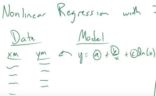
I want to be perfectly and totally clear: The above model is linear. You can and in fact should use linear regression to solve this. All you need to do is create two more columns in your data–one being the reciprocal of x, and another being the natural log of x–and include those as features in your regression. If you use a nonlinear model to solve this, I will sneak into your house at night and uninstall Python and R off your computer.

$y = \beta_0 + \beta_1 z_{i,1} + \beta_2 z_{i,2} + \epsilon_i$

$z_{i,1} \equiv 1/x_i$

$z_{i,2} \equiv \textrm{ln}(x_i)$

The point here is that linear models do not require that all the variables in your data are explicitly linear. All that is required is that each term can be expressed linearly, i.e. a summation of parameters multiplied by some variable. You can easily accomplish this by “preprocessing” your data in machine learning terms, or “not being lazy” in statistics terms.

I’m sorry for being a little sassy about this. And I’ll be real with you: the truth is it’s not always as easy as “just transform the data to a linear form” because you don’t always know what the underlying process for your data is. In those cases where the data generating process is unknown, it can be hard to tell if your data can be transformed into a linear model in a way that makes sense. It requires some creativity and elbow grease, and sometimes it doesn’t pay off.

But on the flip-side, too often the default mode of thinking is to see nonlinear data and assume the model should therefore be nonparametric or nonlinear instead of thinking about whether the data can or should be transformed into a linear model. All I’m asking of people is to consider that the latter is also a great option!

In fact, all of the following seemingly nonlinear functions can be estimated with a linear regression and proper data transformations:

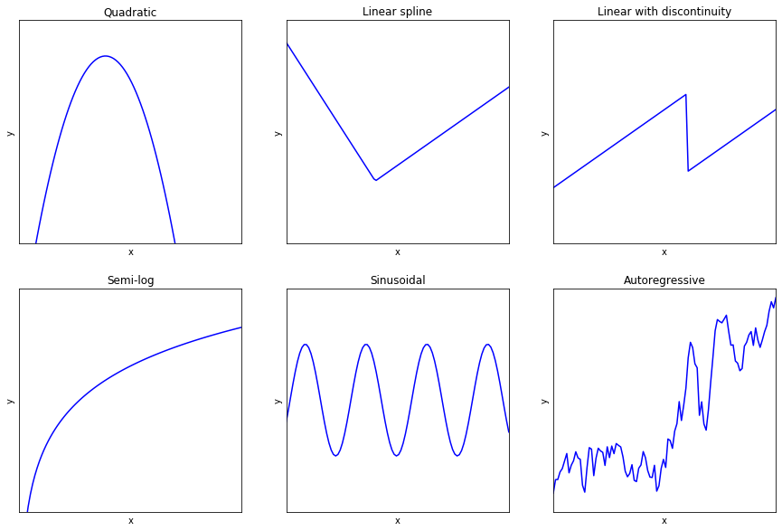
Note that some of these functional forms:

Make certain assumptions about the error term (e.g. semi-log form models assume that errors are multiplicative in the exponential form, and are only additive in the semi-log form);
Require large-sample asymptotic properties for consistent estimates (e.g. autoregressive processes, which are not strictly exogenous);
Require tuning a hyperparameter (e.g. splines and discontinuities require finding where the disjointed component is; autoregressive processes require tuning the number of lags);
Require additional testing (e.g. the autoregressive process might have a unit root);
Cannot be combined cleanly with other methods (e.g. autoregressive terms with fixed effects produce very biased parameters with OLS).

But none of this data requires you to deviate from OLS, as long as you are willing to transform your data. For example, fitting quadratic data simply means making a new column in your data that is $x^2$ , and including that in your regression. Sinusoidal models require three features: $\beta_1 x$ , $\beta_2 \textrm{sin}(x_i)$ , and $\beta_3 \textrm{cos} (x_i)$ .

How do independent variables interact with one another in a regression?

A friend of a friend asks this question in the job interviews they conduct: “If you add a new variable to a [unpenalized] linear regression, and one of the other parameters changes, what does that indicate about the variables?”

Believe it or not, some otherwise smart people can’t answer this question, even though the question is fundamental to data modeling in general. I suspect one reason why is because machine learning techniques let you avoid considering this question in the day-to-day. At worst, adding more variables does nothing to improve the predictive accuracy of your model and can only make your model predict better. Some ML methods do the feature selection for you, and often in ML you often don’t look at or really care about the parameters. So it’s easy to forget how they work.

The simple answer to this question is that a change in one of the other parameters means the variables are correlated (geometrically, you could say that the variables are not orthogonal).

The less simple answer to this question is the Frisch-Waugh theorem.

Back in the stone age, before computers were blazing fast, calculating regressions took a very long time. This had various implications. First, it was important you knew every single detail about the regression you’re calculating before you do one–you only got one regression, and it had to count! Second, understanding the properties of OLS and regressions was extremely important because some of those insights could make your job a lot easier. Instead of taking two weeks to calculate one regression, maybe a little trick could make it take one week instead. Furthermore, you had to actually do abstracted mathematics to derive those properties instead of brute-forcing your way into those insights because, you know, there were no computers.

One question you might have been concerned about back in ‘ye olde days was the question of which is better:

Detrending each variable (i.e. removing the time-related component from each variable) then performing a regression on the detrended variables.
Adding time as a variable to your model without detrending.

In 1933, Ragnar Frisch and Frederick Waugh proved that these are actually the same thing (as far as your not-time-related parameters are concerned). In other words, including time as a variable detrends the other parameters. Hooray, now calculating regressions is marginally easier without blazing fast computers! (Michael C. Lovell generalized this theorem to all subsets of variables, not just time trends, and so the theorem is sometimes called the Frisch-Waugh-Lovell theorem.)

Frisch-Waugh is basically a microcosmic version of the geometric intuition that OLS orthogonally projects $\mathbf{y}$ onto the subspace spanned by the columns of $\mathbf{X}$ to get you to $\hat{\boldsymbol y}$ . (See footnote 1.)

In slightly less jargony terms: each column of $\mathbf{X}$ explains some component of the variation of $\mathbf{y}$ . If two columns are not orthogonal to one another, then each column explains a portion of the variation that is orthogonal to the other. (See footnote 2.) Of course, this brings us full circle: when each column is orthogonal to all the others, then dropping one doesn’t affect the others.

Conceptualizing linear regression as a system of equations (instead of one single equation).

Did you know that $\left(\mathbf{X}^{\mathsf{T}} \mathbf{X} \right)^{-1} \mathbf{X}^{\mathsf{T}}$ is the pseudo-inverse of $\mathbf{X}$ ? It’s an “inversion,” so to speak, because multiplying it by $\mathbf{X}$ gets you the identity matrix, $\mathbf{I}_N$ .

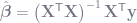
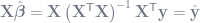
This so-called “pseudo-inverse” of X can be found in the OLS estimate, $\hat{\boldsymbol \beta} = \left(\mathbf{X}^{\mathsf{T}} \mathbf{X} \right)^{-1} \mathbf{X}^{\mathsf{T}} \mathbf{y}$ . This is not a coincidence.

Do you remember solving systems of linear equations in high school precalculus? Or college linear algebra? At first you do the equations by hand, perhaps with the Gauss-Jordan algorithm. Then you learn that there is a matrix form of the system, $\mathbf{A x} = \mathbf{y}$ , where $\mathbf{A}$ is a square matrix. Then you learn that this system can be solved by multiplying both sides by the inverse of $\mathbf{A}$ , i.e. $x = \mathbf{A}^{-1} \mathbf{y}$ .

Look familiar? Yep, the OLS estimator is simply your feature space (pseudo-)inverted then multiplied by the dependent variable vector.

Anyone who uses Matlab (godspeed, you brave souls) is already intimately familiar with this: in Matlab, you don’t solve OLS with a function called “regression” or anything like that. Instead, to solve for Xb=y, you “divide” $\mathbf{y}$ by $\mathbf{A}$ from the left to get $\mathbf{b}$ , which in Matlab terms is b = y\X (\ is dividing from the left, / is dividing from the right). (See footnote 3.)

This is a very different way of thinking about OLS than you’re probably used to if you’re using R, Python, or Stata, which is precisely why I’m bringing this up. In most statistical programs, we think of $\hat{ \boldsymbol \beta}$ as the vector that provides the line of best fit for one linear equation with unknowns $\beta_{0}, ... \beta_{K}$ , and $\mathbf{X}$ contains all the possible values of that single equation. In this framing, we think of $\hat{ \boldsymbol \beta}$ as minimizing the squared errors for one equation.

In the way that Matlab frames the problem, $\hat{ \boldsymbol \beta}$ is not a best fit for one linear equation that takes multiple values; instead, it is a solution to a system of N quantity of linear equations where each row of $\mathbf{X}$ represents what each equation in the system looks like. The difference is subtle, but tangible.

This is not always the best way to conceptualize linear regression, but it’s important to have it in your toolkit. For example, understanding this way of thinking can help you better conceptualize other statistical methods such as the generalized method of moments, which (at least for me, personally) makes more sense with the “system of linear equations” framing.

What’s the easiest way to understand why and how lasso and ridge behave differently?

Lasso and ridge are two ways to add penalization (a way to regularize your model, i.e. reduce variance and increase bias) to a linear model. The mathematical difference between lasso and ridge is pretty straightforward: lasso penalizes by the sum of the absolute values of the parameters; ridge by the sum of squares). However, thinking about the implications of this behavior can be tricky, and isn’t often clearly explained.

$\hat{\boldsymbol{\beta}}_{\rm lasso} = {\rm argmin}_\beta \sum_{i=1}^n (y_i - \mathbf{z}_i ^{\rm T} \boldsymbol{\beta} )^2 + \lambda \sum_{j=1}^K | \beta_j |$
$\hat{\boldsymbol{\beta}}_{\rm ridge} = {\rm argmin}_\beta \sum_{i=1}^n (y_i - \mathbf{z}_i ^{\rm T} \boldsymbol{\beta} )^2 + \lambda \sum_{j=1}^K {\beta_j}^2$

The most useful way to think about lasso and ridge in general is to think about extremes. For example, when the penalty $\lambda$ is 0, you get OLS, and when $\lambda$ approaches infinity, the only way to not overwhelm the model is to set all the parameters $\beta_j$ to 0. (Except the intercept, which is usually excluded.) This is true of both ridge and lasso. (Also, do note that parameters in both ridge and lasso should be normalized, otherwise your model will not be scale invariant.)

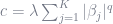
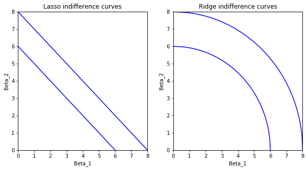
As for the differences between ridge and lasso, you can also think about those in terms of extremes. For example, think of all the points where the penalty term is some constant, $c = \lambda \sum_{j=1}^K |\beta_j|^q$ , for q=1 (lasso) or q=2 (ridge). In consumer theory in economics, we’d call this an “indifference curve,” i.e. the set of all points where an agent is indifferent between two (or more) allocations of goods. A word of warning, this is not a term that is actually used in machine learning or constrained optimization, but this nomenclature help understand what’s going on.

Points along each curve are where the penalty is constant.

Note with ridge regression how the slope changes: On the uppermost curve, as $\beta_1$ gets closer and closer to 8, the slope approaches infinity. This means that even if both parameters are pretty highly correlated, it gets harder and harder to justify reducing $\beta_2$ to zero as you move along the curve, because the trade-off from reducing $\beta_2$ just to increase $\beta_1$ gets more and more severe the more that you approach zero.

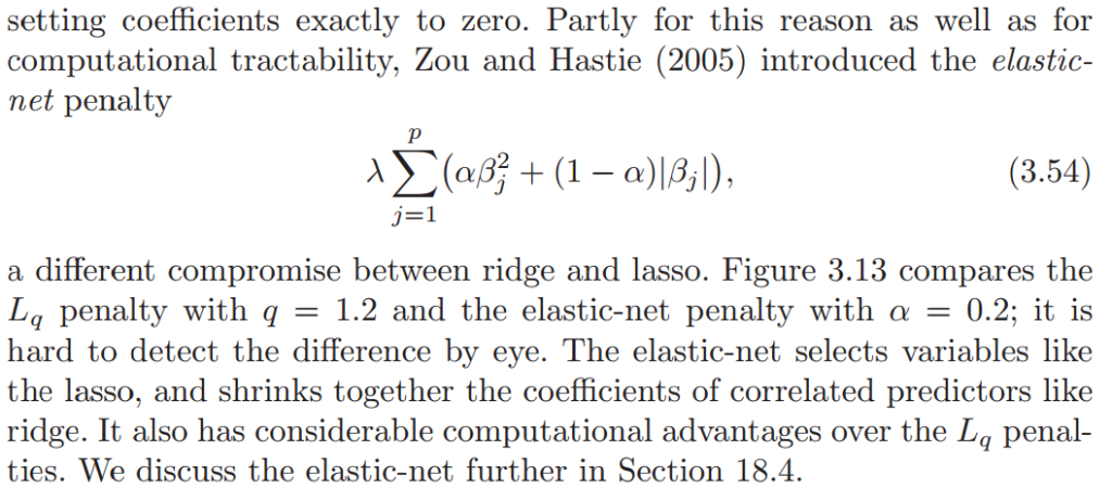
Lasso does not behave like this. Going from $\beta_1$ = 7.99 to 8 along the indifference curve gives you just as much “breathing room” in the penalty term as you’d get when moving from $\beta_1$ = 3.50 to 3.51. In fact, this behavior is why lasso allows for “feature selection”: If $\beta_1$ eclipses $\beta_2$ in predictive power and both are correlated, with lasso it makes no sense to take a little bit from both because the rate of change between the two penalties along this indifference curve is constant. If your penalty is the L2 norm, though (i.e. ridge), you must end up with some combination of the two parameters.

The only question remaining is: how do you choose between ridge and lasso? Honestly, I’m not so sure myself. Some would argue the real answer to this question is to just use elastic net, which is essentially a middle ground between ridge and lasso, but without compromising lasso’s feature selection property. (See footnote 4.) Worst comes to worst, when tuning the $\alpha$ hyperparameter, you end up with $\alpha = 0$ , which is just lasso. But if alpha > 0? Then you have a model with more predictive power! What’s to lose?

Can penalized parameters be used for causal inference?

Penalized regressions (ridge and lasso) will predict better out of sample than plain ‘ol ordinary least squares because of the bias-variance trade-off. The TLDR is: totally unbiased estimates have more variance, which means they are more sensitive to fluctuations in the data you ran the model on. So when it comes time for the model to “see” previously unseen data, that higher variance can cause your model to be a bit off. If you are not regularizing your predictive models (via penalization, in the case of linear regression), then you are probably doing something wrong.

Based on that fact, it seems unintuitive to suggest that although penalized parameters are superior for predictive purposes, they’re also inferior for causal inference. After all, if penalization makes the model fit better out of sample, doesn’t that mean it’s the more “correct” model? And isn’t a more “correct” model better for all purposes–including inference?

This seems to be the view of some data science trolls in my Twitter mentions who keep telling me that no regression should ever be left unpenalized. And it is–in a word–wrong.

In more than one word: there are two ways to think about why penalized parameters cannot be used for causal inference.

The first way to think about this is similar to the intuition behind omitted variable bias (OVB). Imagine that we’re measuring wages ( $\textrm{wage}_i$ ) as a function of education, ( $\textrm{educ}_i$ ). Our linear regression is:

$\textrm{wage} = \beta_0 + \beta_{\textrm{educ}} * \textrm{educ} _i + \epsilon_i$ .

But what if wage and educ both correlate with something not included in the regression equation, such as innate skill ( $\textrm{skill}$ )? (Note: innate skill is hard to measure, which could be why it wasn’t included in the first place.) Recall the discussion of the Frisch-Waugh theorem above to think about how including or excluding this variable affects the coefficient for education, $\beta_{\textrm{educ}}$ . Without including a term for innate skill, $\beta_{\textrm{skill}} * \textrm{skill} _i$ , the coefficient for education $\beta_{\textrm{educ}}$ picks up some of the effect that innate skill has on wages. This means the parameter is overstating how much education affects wages. So the parameter is not an accurate metric of causality until the OVB is resolved.

What does this have to do with penalization? Well, let’s say you find a way to accurately measure skill and include it in your regression, alongside 10 other variables, but then you penalize the model. Penalization will tend to favor variables that correlate with other independent variables: if one variable can account for most of the variation but also correlates with other variables (let’s say, for example, $\textrm{educ}$ ), then slapping a large coefficient on $\textrm{educ}$ and small coefficients on the others puts less stress on the penalty term (and is thus favored by the penalized regression estimator) than the reverse of putting large coefficients on the others and a small coefficient on $\textrm{educ}$ . In other words, we’re back to square one: penalization resulted in us omitting variation caused by other variables (i.e. we have OVB), and $\beta_{\textrm{educ}}$ is still too large relative to the other coefficients.

UPDATE [December 6, 2019]: I had been meaning to make this update for a while, but I had put it off until now. A previous version of this post referenced two arguments for why causal inference requires unpenalized parameters. The first of these arguments (OVB) is, as far as I can tell, sound, and can be read above. The second argument was fallacious, and has since been removed. The second argument’s flaw was that it effectively said that parameters should not only be norm-unpenalized, but made unbiased in general. Bias and norm-penalization are not interchangeable, and as such, I fell into a trap. An estimator, even a causal one, can make a trade-off between precision and accuracy, and it may be the case you can find a biased estimator that has a lower mean squared error than an unbiased one, and that estimator may be preferable in some cases.

Footnotes

Footnote 1

Recall that $\hat{ \boldsymbol \beta}$ is the OLS estimate of the regression equation, and that has its own formula: $\hat{\boldsymbol \beta} = \left( \mathbf{X}^{\mathsf{T}} \mathbf{X} \right)^{-1} \mathbf{X}^{\mathsf{T}} \mathbf{y}$ . Also recall that when you run a predict() function to calculate predicted values of y (i.e. y-hat, or $\hat{ \boldsymbol y}$ ), you are multiplying the X’s by your estimated parameters (i.e. beta-hat, or $\hat{ \boldsymbol \beta}$ ); in other words, $\hat{\mathbf{y}} = \mathbf{X} \hat{\boldsymbol \beta}$ .

Finding the best fitting values of your linear regression is a “projection” of $\mathbf{y}$ onto $\hat{\mathbf{y}}$ .

A projection is any linear transformation that is “idempotent.” A transformation matrix that is “idempotent” is one where $\mathbf{P}^2 = \mathbf{P}$ . In other words, if applying a transformation two, three, four times onto the same data does not make it different than the first time, that counts as a projection.

When we combine the equations for the OLS estimate $\hat{\boldsymbol \beta}$ and the fitted values $\hat{\mathbf{y}}$ , we get the following relationship:

$\mathbf{X} \hat{\boldsymbol \beta} = \mathbf{X} \left( \mathbf{X}^{\mathsf{T}} \mathbf{X} \right)^{-1} \mathbf{X}^{\mathsf{T}} \mathbf{y} = \hat{\mathbf{y}}$

The matrix that explicitly gets you from y to y-hat has a special name: (you guessed it) the projection matrix, $\mathbf{P} \equiv \mathbf{X} \left(\mathbf{X}^{\mathsf{T}} \mathbf{X} \right)^{-1} \mathbf{X}^{\mathsf{T}}$ .

The concept of the projection matrix and its cousin, the annihilator matrix $\mathbf{M} \equiv ( \mathbf{I}_N - \mathbf{P} )$ , help you solve the Frisch-Waugh theorem. I highly recommend the analytical questions in chapter 1 of Hayashi’s Econometrics textbook for a thorough overview of this theorem and the math behind it, if you have access to this text.

Footnote 2

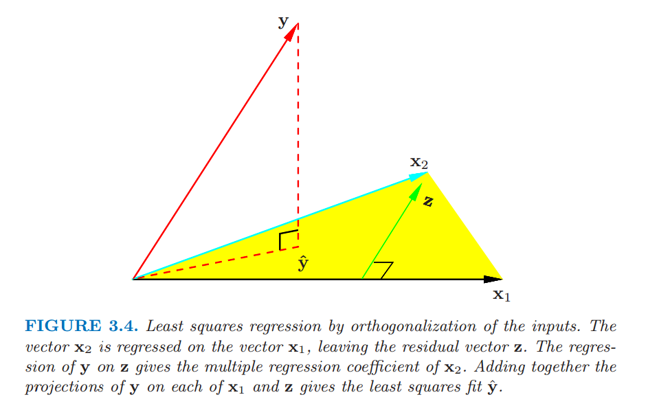
Frisch-Waugh is commonly taught in econometrics and statistics by name, ultimately to inform some of the algebraic intuition behind omitted variable bias. The Elements of Statistical Learning (TESL), a machine learning textbook, effectively teaches Frisch-Waugh’s intuition without actually calling it such, and the way it does so is pretty cool! Instead of splitting $\mathbf{X}$ into two separate column matrices as is done in econ texts, TESL teaches multiple linear regression as a series of univariate linear regressions, and the orthogonal components $z$ of each additional column $\mathbf{x}_i$ added to the regression on $\mathbf{y}$ is the additional contribution of column $\mathbf{x}_i$ to the regression. This eventually dovetails into to a QR decomposition interpretation of the OLS. Multicollinearity is also explained as when $\mathbf{z}$ is small.

Footnote 3

Note that even in Matlab, no pseudo-inversions are being explicitly calculated to get your OLS solution, since that would take way too long. Matlab uses the QR decomposition $\mathbf{X} \equiv \mathbf{QR}$ , which eventually gets you to $\mathbf{R} \hat{\boldsymbol \beta} = \mathbf{Q}^{\mathsf{T}} \mathbf{y}$ . Typically the generalized minimal residual method (GMRES), which uses Krylov subspaces, is most commonly used to solve linear models in other languages.

Footnote 4

I expressed penalization generally as $\lambda \sum_{j=1}^K |\beta_j|^q$ , where q=1 is lasso and q=2 is ridge. It’d be intuitive to guess that 1<q<2 is therefore elastic net. This is almost true, but not 100% true–the difference is that elastic net has “sharp” corners, whereras the $L_{1<q<2}$ norm does not. This is what allows elastic net to have feature selection; if the corners were not sharp, then there would be some point in the neighborhood of one of the intercepts where the slope approaches infinity or 0, which is the reason why ridge regression cannot perform feature selection. Via TESL:

Some Things You (Maybe) Didn’t Know About Linear Regression

Some Things You (Maybe) Didn’t Know About Linear Regression

Linearity is not that restrictive of an assumption.

How do independent variables interact with one another in a regression?

Conceptualizing linear regression as a system of equations (instead of one single equation).

What’s the easiest way to understand why and how lasso and ridge behave differently?

Can penalized parameters be used for causal inference?

Footnotes

Footnote 1

Footnote 2

Footnote 3

Footnote 4

Recommend

Scikit-learn’s Defaults are Wrong

The difference between me and you is that I’m not on fire

Blog_Code/ROI-fot-hot-spots-policing.ipynb

Conjoint Analysis of Crime Rankings | Andrew Wheeler

Papers

SpreadSheet_WDD_HarmExample.xlsx

weighted displacement difference

Mapping Attitudes Towards the Police at Micro Places

Analyzing suspected collusion among bidders

scatterplot

About Joyk