Mapping Attitudes Towards the Police at Micro Places

Objectives

We examine satisfaction with the police at micro places using data from citizen surveys conducted in 2001, 2009 and 2014 in one city. We illustrate the utility of this approach by comparing micro- and meso-level aggregations of policing attitudes, as well as by predicting views about the police from crime data at micro places.

Methods

In each survey, respondents provided the nearest intersection to their address. Using that geocoded survey data, we use inverse distance weighting to map a smooth surface of satisfaction with police over the entire city and compare the micro-level pattern of policing attitudes to survey data aggregated to the census tract. We also use spatial and multi-level regression models to estimate the effect of local violent crimes on attitudes towards police, controlling for other individual and neighborhood level characteristics.

Results

We demonstrate that there are no systematic biases for respondents refusing to answer the nearest intersection question. We show that hot spots of dissatisfaction with police do not conform to census tract boundaries, but rather align closely with hot spots of crime. Models predicting satisfaction with police show that local counts of violent crime are a strong predictor of attitudes towards police, even above individual level predictors of race and age.

Conclusions

Asking survey respondents to provide the nearest intersection to where they live is a simple approach to mapping attitudes towards police at micro places. This approach provides advantages beyond those of using traditional neighborhood boundaries. Specifically, it provides more precise locations police may target interventions, as well as illuminates an important predictor (i.e., nearby violent crimes) of policing attitudes.

Targeting crime at micro place hot spots has become the norm for modern police departments (Weisburd and Telep 2014), and overall, hot spots policing appears to effectively reduce crime (Braga et al. 2012). However, crime is not the only phenomenon of interest to police. Though it is well-known that policing requires cooperation from individuals in the communities they serve, we understand little about how attitudes towards the police may be distributed at the microlevel, nor what microgeographic factors influence policing attitudes. This is an important oversight because understanding attitudes at the microlevel may be useful both to practitioners who desire to target interventions to small areas of discontent, as well as to researchers aiming to understand how local characteristics influence people’s perceptions of the police. Moreover, examining sentiment toward police at the microlevel may illuminate patterns of satisfaction that are masked by the neighborhood-level aggregations typical in both evaluation and theory-centered research.

Treating smaller units as indicative of neighborhood context may also be more consistent with residents’ own perceptions of their neighborhoods (Slovak 1986; Smith et al. 2000). Indeed, in two of the surveys used here, residents were asked what they considered their neighborhood to be: their block, a few blocks away, a section of the city, or the whole city. Most respondents in each survey reported that they viewed their neighborhood as comprising the few blocks nearest their residence (see Fig. 1).

Fig. 1

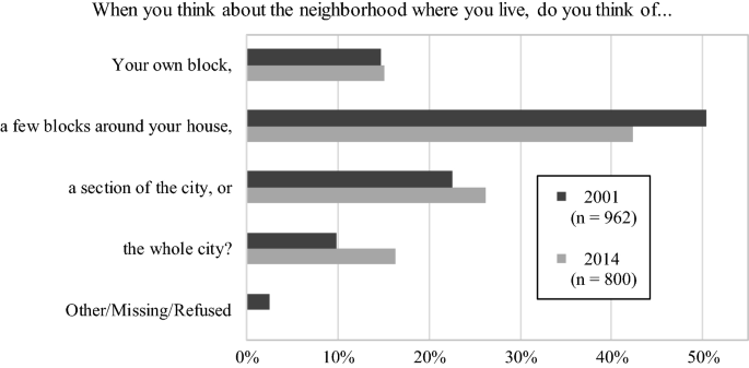
Resident perceptions of what encompasses their neighborhood from two different resident surveys—2001 versus 2014

Full size image

In this study, we illustrate the potential that mapping attitudes toward police at micro places has for informing police interventions as well as for theoretical development. Specifically, using data from three surveys of a mid-sized city in the northeastern United States, conducted in 2001 (Survey 1; N = 962), 2009 (Survey 2; N = 423), and 2014 (Survey 3; N = 800), we provide empirical evidence regarding microlevel hot spots of negative sentiment toward the police. The analysis has three major aims. First, we consider the feasibility of this methodological approach, with particular attention paid to potential concerns about geocoding and survey non-response. Second, we assess the nature of microlevel attitudes toward police by producing descriptive maps and examining how microlevel attitudes compare to related spatial phenomena (census tract-level policing attitudes as well as microlevel crime patterns). Third, we consider the degree to which nearby violent crimes predict individuals’ attitudes toward the police, and demonstrate that nearby violent crimes are the strongest predictors of individual-level attitudes toward police, above and beyond individual or neighborhood characteristics.

Citizens’ attitudes toward the police have long been of concern to both practitioners and researchers, and with good reason. Citizens’ satisfaction with the police is an important goal in and of itself. Fostering positive attitudes toward police may also have more practical benefits for police departments. One such attitude towards police is their perceived legitimacy. Citizens who view the police as legitimate—that is, as trustworthy and deserving of the authority that they hold—may be more likely to comply with police directives, to cooperate with police, and to support their local police departments (Mazerolle et al. 2013; Sunshine and Tyler 2003; Tyler and Jackson 2014). More general positive views of the police have also been linked to law-abiding behavior when officers are not present (Sunshine and Tyler 2003; Tyler 1990). Research shows, however, that shifting attitudes toward police in a positive direction may be exceptionally difficult (Skogan 2006a).

Despite this, many policing programs and academic efforts have been aimed at improving or evaluating citizens’ sentiment toward the police, and one of the major themes in both policy and research centered on policing attitudes has been place. In particular, many police interventions with the goal of fostering community cooperation have targeted neighborhoods, police beats, or other similar areas (Higginson and Mazerolle 2014). A large component of community-oriented policing, for example, is to focus efforts at building police-community relations at the neighborhood level (e.g., Skogan 2006b). Other police programs, such as foot patrol and neighborhood watch, are often implemented neighborhood-wide as well (Higginson and Mazerolle 2014; see also Hohl et al. 2010). Just as interventions aimed at reducing crime may be more effective when targeted to smaller geographic areas (Lum et al. 2011), interventions aimed at improving citizens’ attitudes toward the police may be more effective if directed at concentrations of negative sentiment (i.e., hot spots of negative sentiment). Moreover, insofar as a small number of hot spots can create the appearance of a neighborhood-wide problem in data aggregated to the meso-level, interventions based on neighborhood-level maps of citizen sentiment may expend valuable resources in attempting to improve police-citizen relations where there is little problem while neglecting to focus on the areas in which discontent is most concentrated. Monitoring citizens’ attitudes at the microlevel may also help to improve existing hot spots policing techniques. For example, police departments might use information about attitudes at the micro level to select strategies for dealing with hot spots of crime (Haberman et al. 2015; Kochel 2018; Spelman 2004), or to evaluate the effects of hot spots policing on citizens’ attitudes (Weisburd and Telep 2014).

On the academic side of things, researchers have devoted considerable effort to understanding how neighborhood characteristics shape policing attitudes. In particular, research building on social disorganization theory suggests that neighborhood-level factors such as disorder, concentrated disadvantage, and crime affect citizens’ attitudes toward police (Gau et al. 2012; Luo et al. 2017), and that geographic characteristics should be expected to influence attitudes about police above and beyond the individual-level factors such as race, age, or SES. Empirical results, however, have provided only moderate support for this theory. Whereas neighborhood-level variables have been shown to affect attitudes about police net of individual-characteristics, few findings are consistent across studies (see Corsaro et al. 2015; Kirk and Papachristos 2011; Reisig and Parks 2000; Sampson and Bartusch 1998; Slocum et al. 2010; Wu et al. 2009), and some research shows that neighborhood or municipality conditions have no effect on citizens’ views of police (Gau et al. 2012; Taylor and Lawton 2012; Wells et al. 2006). Rather, most of this research points to individual-level characteristics or experiences as being more important than spatial characteristics.

A possible reason for lack of strong or consistent effects for neighborhood-level phenomena in theoretical research on policing attitudes, as in interventions centered on police-citizen relations, is that the spatial unit that is usually considered—the neighborhood—is not optimal. Indeed, criminological research that focuses on neighborhoods as the unit of analysis may fail to detect important microgeographic variation in crime and its correlates (Hipp 2007, 2010; Smith et al. 2000; Weisburd et al. 2012; Weisburd and Majmundar 2018). Similarly, individuals’ attitudes about police may be specific to smaller or more dynamic geographical areas (Hipp and Boessen 2013; Taylor 1997), and aggregating policing attitudes to larger areas may mask important variation and make it more difficult to find relationships between variables, even when such relationships exist (Smith et al. 2000; Steenbeek and Weisburd 2016). Thus, mapping residents’ perceptions of the police at the microlevel, or considering microlevel correlates of policing attitudes, may aid in further developing theory regarding perceptions of the police, particularly compared to research considering neighborhood-level data only. Accordingly, recent research has called for microlevel examinations of policing attitudes (Circo et al. 2018).

In examining patterns of variation in policing attitudes at micro places, we must also consider a related question: why might attitudes about police cluster in ways that do not conform to neighborhood boundaries. We argue that of particular theoretical interest are micro-level patterns of crime, which may influence the formation of policing attitudes in a few ways. That is, insofar as residents of crime hot spots experience frequent crime and disorder at their homes (Solymosi et al. 2015; Zhao et al. 2015), they may be especially likely to hold negative views about police compared to citizens who reside elsewhere (see Luo et al. 2017).

One explanation is that, as researchers have long noted, citizens generally expect police to address crime and disorder, and a failure to do so effectively may lead people to view police negatively (Luo et al. 2017; Skogan 2009; Zhao et al. 2014). Indeed, numerous studies have linked views about police to perceptions of nearby crime and disorder (e.g., Bradford et al. 2009; Lai and Zhao 2010; Van Craen and Skogan 2015). In addition to informing instrumental judgments about police effectiveness, however, residence near hot spots of crime may also shape attitudes toward police based on a heightened fear of victimization, direct or vicarious victimization, or perceptions of social breakdown (Bradford et al. 2009; Circo et al. 2018; Skogan 2009; Luo et al. 2017; Zhao et al. 2015). Of course, when individuals are nearby micro place hot spots of crime those perceptions of victimization, crime, and disorder are likely to be well founded (Kochel 2018).

The emotional effects of residence on or near a hot spot of crime may be also heightened insofar as people have the greatest expectations of safety from crime at their homes (Lai et al. 2017). In contrast to this hypothesis, however, one recent study (Zahnow et al. 2017) found that residential proximity to a recent violent crime was associated with greater confidence in police, although the overall amount of violent crime occurring near one’s residence was not associated with confidence in police.

In addition to shaping perceptions of police directly, residence at hot spots of crime may also influence perceptions of police by affecting the frequency and nature of citizens’ police encounters, as police must frequently respond to crime or engage in preventive measures on hot spot residents’ doorstops. Indeed, research indicates that, even absent of formal hot spots policing programs, policing tends to be more intensive and coercive at hot spots of crime (Lee et al. 2014; Weisburd et al. 2014), and there exist theoretical reasons to expect that increased police activity at hot spots of crime may have a detrimental effect on police legitimacy among residents (Kochel 2011; Ratcliffe et al. 2015; Weisburd et al. 2011). Thus, citizens who reside at hot spots may experience a greater volume of police contacts (whether as suspects, victims, witnesses, or bystanders), which may be, on balance, more negative than police contacts that occur elsewhere.

Given that evaluations of policing attitudes at hot spots have focused only on the effects of programmatic interventions (Ratcliffe et al. 2015; Kochel and Weisburd 2018; Weisburd et al. 2011), rather than contrasting residence on a hot spot to residence elsewhere, little is known about the effects of policing at hot spots on citizens’ attitudes. To our knowledge, no research has yet attempted to map sentiment toward the police at the microlevel across an entire city. Rather, research considering microlevel policing attitudes has tended to measure those attitudes at crime hot spots only (Haberman et al. 2015; Kochel 2018; Ratcliffe et al. 2015). Thus, we do not know how attitudes about police are distributed in micro places where crime is not exceptionally high, nor do we know how the distribution of policing attitudes at micro places compares to neighborhood-level aggregations of police attitudes. Moreover, despite theoretical reasons to expect negative sentiment toward police to concentrate at hot spots of crime, little research has examined local correlates of policing attitudes (but see Luo et al. 2017; Zahnow et al. 2017).

The current study thus aims to address each of these issues in two particular ways. First, we illustrate how one can make maps that identify small areas of dissatisfactionFootnote 1 with police, analogous to maps of hot spots of crime, based on survey measures of attitudes towards police. Second, we predict satisfaction toward police based on micro level measures of nearby violent crime counts while controlling for individual characteristics (e.g., race, sex, age) that have previously been linked to attitudes about police. Using these approaches, we show that hot spots of dissatisfaction are highly correlated with micro level measures of violence in these samples, and that those micro spatial factors appear to be large determinants of satisfaction towards police, even above the individual-level factors.

The city under study is a mid-sized city in the northeastern United States. The city is approximately 70 km2, and the population, which has not undergone any drastic demographic changes in the past 20 years, is under 250,000 but over 50,000 residents. The police department employs under 300 sworn officers. Compared to similarly-sized cities, the city under study has high Uniform Crime Report violent and property crime rates, though the temporal pattern of crime has followed a similar trajectory to most of the United States (i.e., crime rates rose until around the mid-1990’s and have been falling since that period). Note that we maintain anonymity of the site throughout the analysis by generalizing the census tract polygons as well as the border of the city. This procedure maintains continuity between tracts, and also largely maintains straight boundary lines between the original census tract areas. This property is important, as we will later show how several of hot spots of negative community sentiment straddle the borders of census tracts.

To capture citizens’ perceptions of police, we used data from three city-wide surveys. The first was conducted by phone in 2001. Tax records were used to identify and sample at least two individuals per street block. Households were then sampled from the 1924 city blocks that had at least one residential phone number. We sampled two households from blocks with 20 or more households (20% of all blocks) and one household from each of the remaining blocks (80%), for a total of just over 2300 surveys. One adult in each household was interviewed. We conducted interviews with 962 respondents (a response rate of 42%) who represented 866 (45%) of the blocks.

The second survey was conducted by mail in 2009. We drew a random sample of households (again via tax records) stratified by the police department’s nineteen patrol area boundaries. Each patrol area sample of 120 households was drawn to represent apartments and one- to three-family residences proportionately. The sample size was predicated on a response rate of 40%, which had been achieved in some surveys of this kind, using what is known as the “Dillman method” (Grott and Albright 2004; see also Dillman 1978). Between November, 2009 and February, 2010, we mailed three waves of surveys to 2270 households. Surveys included an introductory letter and a postage paid return envelope, and each survey was marked with a numeric code that enabled us to (1) track survey returns and remove households from which responses were received from subsequent mailings, and (2) compute response rates by our sampling strata so that appropriate sampling weights could be applied in analysis of the data. The final sample included 423 returned surveys, yielding an overall response rate of 18.6%, much lower than originally projected. The Wave 1 and Wave 2 mailings produced 39 and 41% of our overall sample, respectively, while the Wave 3 mailing generated only 19% of the final sample, despite the financial incentive we included.

The third survey was conducted in 2014 by phone by a professional survey firm. Zip-codes that had higher amounts of police contacts were purposefully oversampled. For this survey, the survey firm called phone numbers for land-lines until a set number of surveys had been collected (in this case, 800 responses). As such, the exact response rate is not available.

Each survey included measures of respondents’ Satisfaction with Police. Specifically, we asked respondents, “Overall, how satisfied are you with the quality of police services in your neighborhood?” Responses were given on a four-point Likert scale (1 = very satisfied, 2 = somewhat satisfied, 3 = somewhat dissatisfied, and 4 = very dissatisfied).

Additionally, each survey measured person-based characteristics for each respondent. Here, we focused on demographic characteristics that are theoretically or empirically relevant to understanding attitudes about police, and coded the measures to allow for consistency across the surveys. Respondents’ race was measured using dummy variables for African-American (Afr. Am) and Other Race, with White as a referent (e.g., Schuck et al. 2008; Skogan 2005; Weitzer and Tuch 2005). Respondents’ sex was measured using a dummy variable for Female (e.g., Reisig and Correia 1997; Skogan 2005). Respondents’ Age (e.g., Reisig and Correia 1997) was coded as a continuous variable and divided by 10 to ease interpretation of coefficient sizes in the analysis. Socioeconomic status (e.g., Schuck et al. 2008; Wu et al. 2009) was operationalized using two dummy variables: Income below $20,000, and Education of less than a high school degree. Respondents’ conventional social bonds and degree social integration (Correia 2010; Ferdik et al. 2014) were measured using four variables: employment status, coded as dummy variables for Unemployed, Retired, or In School, with employed as the referent; marital status, coded as dummy variables for Never Married, and Previously Married (including respondents who were divorced or widowed), with married as a referent; residential instability, coded using a dummy variable for lack of home ownership (Do Not Own Home); the number of adults in the home (Adults in Home); and the number of children in the home (Children in Home).

In addition to drawing data from surveys, we also used police records to measure the number of Part 1 violent crimes from 2001 through 2014 occurring within 300 ms of the nearest intersection to the survey respondent. This distance was chosen for two reasons: first, it is likely near the minimal distance necessary to capture the actual home residence of the survey respondent, and second, counts of violent crime within 300 m had the highest bivariate correlation with attitudes towards police (compared to other distance thresholds between 50 and 1000 m). For ease of interpretation in regression models, the number of Part 1 violent crimes was divided by 300. The overall geocoding hit rate for Part 1 violent crimes was over 98%.

Finally, we also incorporated neighborhood level demographic measures at the 2010 census tract level using the 2011 5-year American Community Survey Estimates. These neighborhood level variables included the proportion of female headed households, the proportion of families living in poverty, the proportion of individuals who moved within the prior year, and the proportion of minorities (including Hispanics). Using the Part 1 violent crimes, the violent crime rate per 1000 residents at the census tract level was also calculated.

An important aim of the current study is to demonstrate the feasibility of mapping sentiment toward the police at microplaces. In this section, we discuss our geocoding methods, with particular attention to the geocoding hit rate and potential biases introduced by respondents refusing to disclose where they lived. We also address potential concerns raised by the fact that the survey methodology differed across the three surveys used in this study. The use of multiple surveys presents confounds when evaluating differences between waves but allows us to compare different survey modes for collecting microlevel spatial information.

In each survey, respondents were asked, “Because we need to know the general area where you live, would you please tell me the name of the street you live on?” If the respondent provided an answer to this question, they were also asked, “And would you please tell me the name of the street that crosses that street at the corner nearest your home?” Together, these questions provided the self-reported nearest intersection to each respondent’s residence. In Survey 1, we were additionally able to use the parcel location that was sampled to provide the nearest intersection for respondents who did not answer the questions. Table 1 displays the geocoding hit rates for respondents in all surveys.

In all, we were able to geocode 83% of all respondents across the three surveys. Note that this is lower than typical geocoding hit rates for crime incidents. Although Ratcliffe (2004) suggests a minimum bound of 85%, the majority of contemporary analyses using crime data have much higher geocoding hit rates, often exceeding 95%. Failure to geocode responses typically occurred because the respondent refused to answer the questions (11% of all responses). Indeed, when individuals who refused to answer are excluded from the sample, the total geocoding hit rate is 92%. The refusal rate was lowest in Survey 2 (6%) and highest in Survey 3 (26%). The refusal rate for Survey 1, had we not used the address sampled in cases in which respondents did not supply the nearest intersection, would be 14%. A second common reason for geocoding failure was respondents giving a location outside of the city. This error occurred most frequently in the most recent telephone survey (Survey 3). Specifically, whereas the number of respondents outside of the city was negligible in Surveys 1 and 2, 8% of Survey 3 respondents did not live in the city. This is likely due to sampling at zip-codes, which do not conform perfectly to city boundaries (Grubesic 2008). Thus, using a sampling frame based on zip codes is likely to be less efficient than the other methods for gathering data for a particular city. Finally, some respondents were not geocoded because they gave ungeocodable intersections (e.g., two parallel streets). However, errors of this type were rare.

Overall, the surveys provided good coverage of the city. In total, there were 832 unique intersections for the 1804 geocoded survey responses. Of these, 385 intersections only contained one survey response, but the remaining 447 intersections had between two and twelve responses. This coverage of the city, even in areas with high crime, persisted for each survey wave. In Surveys 1 this was intentional via the sampling design. This was not the case with Surveys 2 and 3, which were stratified by larger patrol areas and zipcodes respectively. Thus, even though it is challenging to collect survey responses in high crime microplaces (Haberman et al. 2015), we find that our method of geocoding provides usable data citywide.

Figure 2 displays a kernel density estimate of the survey responses across the city (a point map is avoided to maintain anonymity of both respondents as well as the city under analysis). While the density is not entirely even over the study area, it generally corresponds to the areas with the majority of residences in the study area, as well as illustrates oversampling in high-crime areas (as subsequent figures will show). The area with the lowest density in the upper portion of the map corresponds to an area with both more commercial land use and a large park.

Fig. 2

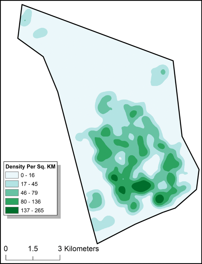
Kernel density estimate of the locations of survey responses across the study area. Displayed are densities per square kilometer (Sq. KM)

Full size image

Table 2 shows the demographic differences between the individuals who we were able to geocode compared to those we were unable to geocode across the three samples. This provides evidence that the respondents who we were unable to geocode did not differ substantively from those who were included in our geocoded sample. The largest difference is in respondents’ education: whereas 24% of geocoded respondents had less than a high school education, 34% of non-geocoded residents fell into that category.

Table 2 also contains demographic information for the respondents we were able to geocode in each survey. We note that each sample was increasingly older (ranging from a mean age of 47 in Survey 1 to a mean age of 57 in Survey 3) and each sample had an increasing proportion of African-American respondents (from 14% in Survey 1 to 27% in Survey 3). Additionally, the proportion of unemployed respondents increased across samples, as did the proportion of respondents making less than $20,000 per year. The city has not experienced a dramatic increase in the African-American population between the 2000 census (28%) and the 2010 census (30%). Neither did it get older, with a median age of 31.4 in 2000 and a median age of 30.8 in 2010. Thus, the differences across the samples are likely an artifact of differing survey methodologies (e.g., the oversampling of some zip-codes in 2014) or changes in groups’ propensity to respond to surveys over time.

As such, we take steps to address potential biases resulting from the use of differing survey modalities. First, we demonstrate that despite these demographic differences, levels of satisfaction with the police are similar across the surveys. Figure 3 shows the responses to this item across the three surveys. More than 80% of the respondents reported being very satisfied or somewhat satisfied with the police in each survey. Additionally, we show in subsequent analyses that when the data are disaggregated, the surveys produce similar microlevel maps of sentiment toward the police (“Appendix C”). In the correlational analyses, we include fixed effects for year in each regression model to ensure that no single survey drives the results.

Fig. 3

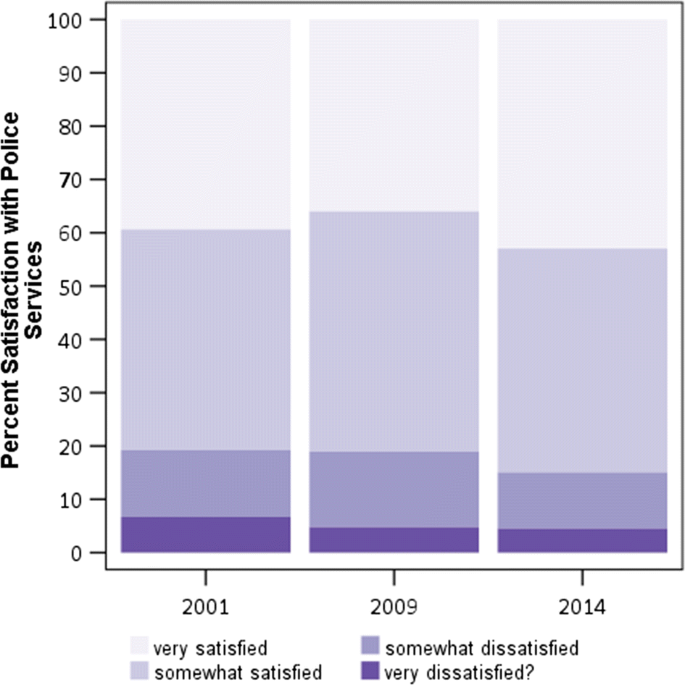
Percent satisfied across different surveys years

Full size image

We used the geocoded data to perform two sets of analyses. The first part of the analysis is descriptive and examines the distribution of respondents’ sentiment toward police at micro places across the city, as well as how micro-level sentiment toward police compares to larger aggregations of sentiment (i.e., census tracts). In this part of the analysis, we also compare the spatial distribution policing attitudes and violent crime at the micro-level. Second, we conduct multiple regression analysis to explicitly assess whether crime near respondents’ residence shapes their micro-level attitudes toward police.

Beginning with the descriptive analyses, we estimate the average sentiment toward police at micro places using inverse distance weighting. This method takes a set of quantitative data and calculates the weighted average at control locations using the following formula (Slocum et al. 2005: p. 274):

The original n observations of Z (e.g. the original survey responses on a 1–4 scale) are indexed by i. For each observation, the distance between that measurement and the control location is calculated and labeled as d. Taking the inverse of this weight is accomplished by the − k power term (most frequently using the 2nd power, providing the inverse of the distance squared, which we also use here). Once the distance weights are estimated, taking the weighted average over the sample is no different than using sampling weights. Inverse distance weighted estimates are then obtained at many control locations on a regular grid over the entire city. One can map these averages to produce a smooth isarithmic raster map. This map is a natural analog to a map of hot spots of crime. Indeed, as expected, hot spots of negative sentiment and hot spots of crime (identified via kernel density) have a substantial amount of overlap in this sample.

We next compared the micro-level distribution of policing attitudes to neighborhood level aggregations by aggregating negative sentiment toward the police at the census tract. This part of the analysis demonstrates the heterogeneity of attitudes within areas usually treated as “neighborhoods.” Aggregating the surveys to census areas (or any neighborhood boundaries) was problematic because neighborhood boundaries are almost always defined by streets, whereas survey responses are recorded at intersections. To solve this problem, we used the method suggested by Snijders and Bosker (2012) for cross-classified multilevel data. We duplicated survey responses that fall on a census tract border, and then weighted the duplicated cases by the inverse of the number of tracts they border. For example, if a case fell on the border of two census tracts, it was given a record for each tract, but each survey response was only given a weight of 1/2. If it fell on the border of three tracts, it was given three records and each a weight of 1/3, and so on. This method preserves the aggregate properties of surveys (such as the total citywide average), but allows us to aggregate surveys to census tracts. To calculate which survey responses fell on the borders of census tracts, we buffered the survey intersections by 5 m and included responses located on intersection of those buffers with the census tract dataset.

We also addressed whether individuals’ place of residence matters in how they form opinions towards police, above and beyond individual-level or neighborhood-level characteristics, with an eye toward understanding the effects of residence near areas of violent crime. This is because the observed spatial correlations between attitudes and crime can potentially be due simply to racial or economic segregation. To do this, we fitted a series of regression models predicting sentiment toward the police. The models were based on 1331 complete cases, resulting from the attrition of 473 cases from the 1802 surveys we were originally able to geocode. “Appendix A” contains multiple imputation analysis to attempt to correct for missing data selection (Allison 2002). The imputed effects were very similar to those reported in the complete case analysis, so we only report the complete case analysis in text for simplicity.

We fitted several models to identify characteristics that are theoretically predictive of attitudes towards the police. The first model is a linear regression equation predicting attitudes towards the police as a function of various person-based characteristics (i.e., race, sex, income, education, employment status, marital status, residential instability, and the number of adults and children in the house). We also controlled for the survey year. The model is shown below.

We refer to these person-based characteristics as the vector X_{k} \beta_{k} in further regression models. While the sentiment scale is composed integers of values 1–4, and so an ordinal logistic regression model may be more appropriate (Long 1997), we used linear regression for ease in interpretation of the coefficients, as well as the ability to fit more complicated models that include spatial effects. Given that none of the models produced predictions outside of the 1–4 range, we are reasonably confident they provide valid predictions and effect estimates. As a robustness check, we replicated our final presented model (model 4) as a multi-level ordinal logistic regression equation (Christensen 2015) and found no substantive differences among the results for each model (see “Appendix B”).

Model 2 adds the number of Part 1 violent crimes (from 2001 through 2014) occurring within 300 m of the nearest intersection to the respondent, while still controlling for the person-based characteristics of the survey respondent.

Given that crime shows long term stability at micro places (Curman et al. 2014; Weisburd et al. 2004; Wheeler et al. 2016), using an aggregate measure over the entire time period is appropriate.

For all of the models, we assessed the amount of residual spatial autocorrelation in the models using global Moran’s I (Anselin 1995). Smaller absolute values of spatial autocorrelation in the residuals are more desirable, as effect estimates are potentially biased if the regression residuals are not conditionally independent. To create the null distribution for the global Moran’s I test statistic, 999 random permutations of the data were generated (Anselin 1995). The spatial weights matrix used was based on the distance between intersections, derived from the bi-square kernel at a distance of 2000 m (Fotheringham et al. 2003).Footnote 2 2000 m was chosen by examining the spatial correlogram of attitudes, which had a positive correlation that declined to zero by 2000 m. The bi-square kernel was chosen over the inverse distance because it has a much slower decay than inverse distance weighting, which again appears to be more appropriate when examining the spatial correlogram. Also, since some observations had a distance of zero (i.e., survey respondents listing the same intersection), inverse distance is not defined for those cases. The spatial weights matrix was then row-normalized so that the row sum is equal to 1 in the regression models.

Based on this analysis, we found that Model 1 and Model 2 both had a statistically significant amount of residual spatial autocorrelation. To correct for this, we fitted an endogenous spatial lag model (Model 3).Footnote 3 This model is fitted via maximum likelihood, using the lagsarlm functions in the R package spdep (Bivand and Piras 2015). In the following equations the spatial weights are represented as W.

This model shows that nearby attitudes towards police,\rho, contribute a large amount to the prediction and corrects for residual spatial correlation.

We were also interested in assessing the relative contribution of the effects of local characteristics compared to larger neighborhood-level effects. It may be that the local characteristics are confounded with neighborhood level characteristics. Thus, in our final model we fitted a set of random effect models nesting observations within census tracts and intersections. The observations were expanded to census tracts using the method described previously (to account for some intersections being on the border of multiple census tracts) and the regressions were weighted.

In Model 4 we also included rates of violent crimes (per 1000 population) at the census tract level in addition to the local counts of crime, as well as the previously mentioned demographic variables (percent non-White, percent below poverty, percent of female-headed households with children, and the percent who have moved in the past year). Those covariates are represented as X_{d} \beta_{d} in the model. Finally, we included random intercepts for the intersection, \lambda_{l}, as well as for the census tract that the survey was nested within, \gamma_{n}. This model was fitted using the lmer function in the lme4 R package (Bates et al. 2015).

The Micro-level Distribution of Citizens’ Attitudes

We open with descriptive analysis examining the geographic distribution of citizens’ attitudes toward the police. Figure 4 displays the inverse distance weighted map for all three surveys combined, using the responses on the original four-point scale. Since the responses skew positive, a simple color scheme with bins set at [1,2), [2,3), [3,4) would provide very little variation in the map. Instead, the bins chosen for the map are Fisher’s natural breaks based on the means of the bins—the default in ArcMap (Slocum et al. 2005). This is based on 1700 survey responses, as there was missing data on the attitudes toward police question for 104 of the geocoded responses.

Fig. 4

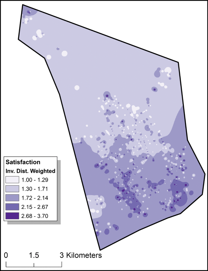
Estimated satisfaction via inverse distance weighting (Inv. Dist. Weighted). Scale is 1—very satisfied, 2—somewhat satisfied, 3—somewhat dissatisfied, 4—very dissatisfied

Full size image

We can see a strong trend in Fig. 4, with more negative responses towards the southern end of the city, and more positive responses towards the northern part of the city. The southern part of the city has several areas that have higher levels of negative community sentiment in smaller areas, denoted by the two darkest shades of purple in the map.

Next, we compare our microlevel data to data aggregated to neighborhoods (operationalized here as census tracts), which are a more common unit of analysis in extant spatial research on citizens’ attitudes toward police (Gau et al. 2012). We also compare the distribution of negative attitudes towards the police to the spatial distribution of violent crime. Figure 5 in the left panel displays the average survey responses across entire census tracts, using 2010 census tract boundaries. The choropleth bin divisions for satisfaction with the police are the same as in Fig. 4. Figure 5 also displays filled contours that show the locations of the two darkest bins (on average over 2.14) for the inverse distance weighted map in Fig. 4 and labels the hot spot clusters previously mentioned. This allows for a direct comparison between the identified hot spots of negative sentiment in Fig. 4 and the tract-level areas of negative sentiment in Fig. 5.

Fig. 5

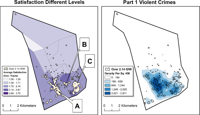
Satisfaction averaged to census tracts (left panel) and overlap of negative attitudes towards the police with Part 1 violent crimes (right panel). The contour areas are those identified by inverse distance weighting (IDW) as having averages above 2.14—so are comparable to the darker purple colored bins in the census tract classification. Three of the hot spot areas are labelled to illustrate how they overlap multiple neighborhood boundaries. Part 1 violent crimes (homicide, rape, robbery, and aggravated assault) are between 2001 through 2014 (n = 16,224). Kernel density estimates are based on 300 m bandwidth with a normal kernel, and are displayed as densities per square kilometers (Sq. KM)

Full size image

While the general spatial trend of the inverse distance weighted map is replicated (areas in the north are blue and areas in the south are red) none of the census tracts in Fig. 5 are given the darkest shade (an average negative sentiment of 2.68 or more) to denote strong dissatisfaction with the police. By contrast, the microlevel map in Fig. 4 displays several of these areas. Thus, averaging to larger neighborhood-sized areas provides less variation than does considering attitudes at micro places, as considerable heterogeneity exists within the census tracts. We can also see that in the tracts that are classified as having the most negative sentiment, the identified areas of concentrated negative sentiment are much smaller and limited to more specific areas using the inverse distance weighted criterion.

It is also important to note that the areas of negative sentiment as identified via inverse distance weighting spill across several tract boundaries. We have labeled three of the hot spot areas of negative sentiment in Fig. 5. Hot spot “A” runs along one main arterial for approximately 3 km and spans six different census tracts. Although these are generalized polygons, the straight borders covered by hot spot A were largely preserved. This hot spot happens to run along a main arterial that defines the boundary of a high crime neighborhood that borders several other neighborhoods. Hot spot “B” is similar in that it runs along a road that forms the border for two census tracts. This road includes a commercial strip with many bars and shops and has a high level of drug selling activity. The largest adjacent census tract is shows a higher negative sentiment, but it also borders one labelled as more neutral. The tract that is labelled as a higher negative sentiment, however, only contains the highest level of negative sentiment along its southern border. Finally, hot spot “C” corresponds to an area within a neighborhood in the southeastern part of the city. This hot spot also spans several census tracts, some of which would be categorized as having neutral attitudes towards the police at the census tract level. Thus, our results suggest that aggregating to the census tract level may not only mask variation within neighborhoods, as discussed previously, but may also provide a misleading picture of community sentiment. That is, each hot spot we identified spanned multiple census tracts and caused large swathes of the city to be erroneously characterized as negative or neutral in their sentiment toward police.

Our final descriptive analysis shows the overlap between areas of high crime and areas of negative sentiment toward the police. The right hand panel of Fig. 5 displays the kernel density estimates of Part 1 violent crimes, with the same contour lines showing the areas of negative sentiment toward the police. The maps show that the negative sentiment hot spots are almost perfectly aligned to the hot spots of violent crime. This reinforces the idea that high crime areas tend to have much higher levels of negative police sentiment—even at the microlevel. The correlation between negative sentiment toward the police and the total number of Part 1 violent crimes (within 300 m of the intersections) is 0.27. The correlation is slightly smaller at the census tract level, at 0.18 for violent crime rates. While the magnitude of these differences is not impressive, variance decompositions from one-way ANOVA estimates 8% of the variance in police satisfaction at the census tract level, but 57% of the variance is at the micro place level (Steenbeek and Weisburd 2016). There is thus much more potential to explain individual level attitudes at the micro place level than there is at the census tract level.

Regression Models Predicting Sentiment toward the Police

We next present linear regression models predicting individual respondents’ attitudes towards police (Table 3). Consistent with the maps presented in the previous section, higher scores correspond to more negative attitudes toward the police in these models. Model 1 includes only person-level characteristics, and shows statistically significant effects for African American, Never Married, and Age/10. (Statistically significant effects with a p value of 0.05 or less are bolded in the table.) African Americans have on average more negative attitudes towards the police, with scores that are .16 higher on average compared to white respondents. Older individuals have more positive attitudes towards the police, with an increase of 10 years in age associated with a change in attitudes towards police of − 0.05. The global Moran’s I statistic is 0.04, which is a reduction from 0.08 for the marginal distribution of attitudes. With a sample size of 1331 cases, however, this is still a statistically significant amount of residual spatial autocorrelation.

Model 2, which incorporates Part 1 violent crimes nearby, shows that when Part 1 crimes increase, attitudes are more negative towards the police. As in Model 2, not married and age of the respondent are statistically significant. The respondents’ race, however, is not. This is not due to multi-collinearity, as the variance inflation factors for all variables are under 2.5. Given a sample size of 1331 cases, and the fact that similar estimates are subsequently replicated in a variety of different model specifications, we have good evidence that the race results are robust for this sample. In this model specification being unemployed has a statistically significant negative effect on attitudes towards police, which runs counter to what might be expected, given those unemployed are more likely to be of a lower socio-economic status.

The Beta column in the regression tables reports the standardized effect sizes.Footnote 4 In terms of standardized effect sizes, the local count of violent crimes is the largest coefficient (β = 0.27), meaning that a one standard deviation increase in the count of local crimes results in a 0.27 standard deviation increase in negative sentiment toward the police. Compared to the standardized effect sizes for African Americans (β = .07) and Age (β = − .09) in Model 1, the effect of violent crimes is much larger than any of the individual-level characteristics even when not controlling for the local counts of crime. The global Moran’s I is further reduced to 0.02 in Model 2, but this is still statistically significant, and is higher than any of the values constructed for 999 random permutations of the data.

Model 3 corrects for the residual spatial autocorrelation by including a spatial lag term. The effect estimates for each of the models are substantively very similar. The effect of violent crimes remains statistically significant and the largest effect in the model. The spatial lag effect, rho, is 0.53, showing a fairly large spillover effect. That is, when predicting an individual’s attitude, attitudes nearby in space are a good predictor net of individual level characteristics. The inclusion of the spatial lag term resulted in there being no statistically significant amount of residual spatial auto-correlation in the model residuals.

Model 4 is a multi-level model, which corrects for spatial autocorrelation by nesting survey responses within census tracts and intersections. Like Model 3, there is no residual spatial autocorrelation in Model 4’s residuals.Footnote 5 In this model the coefficients are similar in direction and magnitude to the prior Models 2 and 3. The standardized effect size for the local violent crime measure is again the largest in the model (β = 0.26), but the neighborhood level violent crime rate is a null effect. The proportion minority in a census tract is a significant predictor of negative sentiment towards the police, with a standardized effect size of 0.18, but whether an individual is a minority is still not a statistically significant predictor of sentiment towards the police. The variance of the random effect for intersections is 0.15, and is very small (less than 0.005) for census tracts.Footnote 6 Like the prior variance decompositions, this suggests that there is much more potential to explain variation in attitudes towards police at the micro level of intersections, as opposed to the within the larger census tract area. As a robustness check we estimated model 4 as a multi-level ordinal regression equation. This model resulted in the same inferences, and is reported in “Appendix B”.

This article demonstrates the feasibility and utility of mapping attitudes toward police at micro places. We showed that significant amounts of variation in policing attitudes exists at the microgeographic level. We also found that the pattern of these attitudes was distinct and not captured by census-tract level data, and that hot spots of negative sentiment toward the police exhibited considerable overlap with hot spots of crime (Sampson and Bartusch 1998). Finally, consistent with research on proximity to violence and disorder (Luo et al. 2017; Zahnow et al. 2017), we also demonstrated that local counts of violent crime were a stronger predictor of attitudes towards police than were individual-level characteristics or neighborhood features.

One of our major questions was about the feasibility of mapping and analyzing surveys at the micro level. We found that we were able to address some of the main concerns resulting from our use of survey data. Despite a relatively high proportion (11%) of respondents being unwilling to provide us with an address, we were able to obtain good coverage of the city. Additionally, individuals’ refusals to answer where they lived did not generate any obvious biases in the survey demographics. Based on this study, we can generally conclude that mapping policing attitudes at the microlevel is feasible using survey data typical of that collected by police departments and researchers.

The current study also has implications for police policy and practice. To begin, a key finding of this study is that negative community sentiment toward police clustered into small hot spots. This clustering may thus have the same practical application for police departments as do hot spots of crime—by concentrating on small areas and smaller numbers of individuals, as opposed to diffusing an intervention to a large neighborhood area, police departments interested in improving community sentiment can make the most effective use of their limited resources. Moreover, the finding that hot spots of negative sentiment crossed neighborhood boundaries suggests that typical methods that aggregate citizen sentiment across neighborhoods should be reconsidered, as police departments that focus their efforts on entire neighborhoods rather than hot spots may expend considerable resources addressing problems where they do not exist while neglecting some of the most serious concentrations of negative sentiment. To the extent that major arterials often form boundaries for neighborhoods, it seems plausible to expect that this aspect of findings would replicate in other cities as well. As a caveat, however, extant research on spatially-focused interventions provide promising, but not definitive, evidence of their efficacy (e.g., Graziano et al. 2014; Hohl et al. 2010), meaning that the ability of police to improve citizens’ attitudes via targeted interventions is far from certain.

The finding that negative sentiment toward police is concentrated in micro places of high crime may also have implications for the selection of strategies to use in hot spots policing (see, e.g., Haberman et al. 2015). Although we did not test the specific theoretical mechanisms linking attitudes about police to crime hot spots (e.g., perceptions of effectiveness, fear of crime, police encounters, etc.), they do suggest that police departments may be well-served by choosing hot spot policing strategies that have the potential to both reduce crime while also improving citizens’ experiences, such as problem-oriented policing (Kochel and Weisburd 2018). Relatedly, the results regarding the concentration of negative attitudes toward police at hot spots of crime may also help to shed some light on extant research examining “backfire” effects of hot spots policing tactics, which typically show that police activity at hot spots has no effect on citizens’ attitudes (e.g., Weisburd et al. 2011; Ratcliffe et al. 2015). If negative attitudes toward police are already concentrated at hot spots prior to a formal hot spots policing program, it may be that an additional police presence of a few hours per week has little effect. Thus, in contrast to previous studies suggesting that police action at hot spots makes little difference to citizens, our study indicates that police departments should pay particular attention to the actions that officers take at hot spots of crime, especially given that citizens with pre-existing negative attitudes toward police are more likely to evaluate police actions unfavorably (Brandl et al. 1994; Rosenbaum et al. 2005). Interestingly, however, ancillary analyses suggested that police stops at hot spots may actually be associated with improved attitudes toward police (although these findings were excluded from the main analyses due to multicollinearity between crime counts and stops that make the finding difficult to interpret). However, future research might further assess the ways in which policing tactics at hot spots may shape citizens’ attitudes toward police.

The study also has implications for theory and future research. A major one is that, demographic characteristics (especially race) are typically considered the strongest predictors of attitudes toward police (e.g., Schuck and Rosenbaum 2005; Silver and Pickett 2015; Webb and Marshall 1995). Indeed, in our individual-level model, respondent race was the strongest predictor of satisfaction with police. However, when we included local spatial characteristics in the models, the effects for race were rendered nonsignificant. Thus, the results indicate that research aimed at understanding the sources of citizens’ sentiment toward the police have been neglecting a powerful determinant of policing attitudes—that is, characteristics of micro places, crime and disorder. A fruitful direction for future research, then, might be to unpack the complex relationships between race, policing, and place, with an eye toward further understanding the role of the characteristics of micro places in shaping policing attitudes above and beyond individual characteristics.

In addition to suggesting that individual-level characteristics may be less important than extant research has typically suggested, our findings also indicate that spatial characteristics may be more important to understanding policing attitudes than previous research has shown. That is, previous research examining attitudes toward police as a function of neighborhood characteristics has largely produced weak and null effects (Corsaro et al. 2015; Gau et al. 2012; Sun et al. 2004; Taylor and Lawton 2012; Wu et al. 2009). Our results suggest, however, that this research has produced mixed findings because the unit of analysis was not ideal for examining these relationships (see Smith et al. 2000), not because spatial characteristics are unimportant. While the correlation between crime and attitudes were similar at the micro and census tract level, the potential variance attributable to attitudes at the micro place level was much larger than at the census tract (approximately 60% vs 10%). Perhaps more importantly, the local count of violent crimes nearby was a strong predictor of attitudes towards police, above and beyond the larger neighborhood level context. As such, a fruitful avenue for future research might be to apply “spatial theories” (Smith et al. 2000) to the distribution of hot spots of sentiment toward the police, as a few recent studies have begun to do (e.g., Luo et al. 2017; Zahnow et al. 2017).

Theoretically, however, the underlying reasons why place matters in how individuals formulate opinions by police are somewhat equivocal. For example, the fact that areas of high crime produce more negative attitudes towards police could be interpreted as though individuals hold police accountable based on perceptions of safety, which may be influenced by either direct or vicarious victimization (Corsaro et al 2015; Circo et al. 2018; Lai and Zhao 2010; Luo et al 2017). However, another interpretation may be that officers behave differently in these high crime settings (Klinger 1997), which may result in more negative perceptions of police (Skogan 2006a), particularly given that individuals who reside at hot spots are likely to have frequent police contact. However, research has shown that how individuals are treated during an encounter is only weakly correlated with how they perceive being treated during an incident (Worden and McLean 2017). Future work may thus be better equipped to tease apart such distinctions by focusing not just on global perceptions of police, but by examining specific interactions and subsequent changes in attitudes based on those interactions (Brandl et al. 1994). Additionally, future research might also aim to assess the roles of fear of crime and victimization as possible mediators of place based predictors of attitudes towards police. In either case, it would appear that micro place based factors should be included in future research assessing public opinions about the police, as this work found that they were stronger predictors of attitudes than traditional demographic characteristics in this sample.

Finally, the results may have implications for research assessing other neighborhood-level attitudinal phenomena. For example, numerous studies have used neighborhood-level measures of collective efficacy or legal cynicism to predict crime rates. Given that both collective efficacy (Silver and Miller 2004) and legal cynicism (Gau 2015) are linked to perceptions of police, however, the current study suggests that spatial variation in these phenomena may be distributed in a similar way. Thus, future research might aim to further understand how other types of criminological attitudes are distributed at the microgeographic level. For example, uncovering “hot spots” of low collective efficacy or high legal cynicism could potentially have implications for neighborhood-based crime control strategies as well as for further developing criminological theory.

Our study has a few limitations that should be taken into account when interpreting the results. The first is that we relied on three surveys conducted independently in different years for various purposes (none of which was the mapping of microlevel attitudes). Because the mode (e.g., telephone, mail) and sampling frames of each survey differed it is likely that our results include more measurement error than would samples from typical multi-wave surveys. Similarly, it is worth noting that there were demographic shifts in the surveys despite no demographic shifts in the population of the city, particularly for Survey 3. Relatedly, surveys 1 and 2 (for which we have data on response rates) had low response rates, typical of phone and mail surveys (e.g., Baruch and Holtom 2008; Curtin et al. 2005). Thus, it is possible that nonresponse created bias in our estimates of hot and cold spots. While this is a problem endemic to survey research, not only to our study, we do urge caution in interpreting the results. Finally, another limitation related to our sampling method is that the data are drawn from a single city only. Thus, it cannot necessarily be assumed that the results in this study will replicate to other cities. Future research might therefore seek to replicate these findings using additional datasets.

In addition to conducting surveys with different modalities, we also conducted surveys over an extended period of time, spanning 13 years from the first to the last. Thus aggregating the results into one map of hot and cold spots could potentially bias the results. We do not believe this to be a strong threat to the findings, however, given that there was overall strong stability in the positive ratings of police. Additionally, we show that survey year was not predictive of attitudes towards the police in the regression results. Individual inverse distance weighted maps for each survey wave (in “Appendix C”) show that the hot spots are mostly consistent over time, but have some volatility due to outliers of negative sentiment. This suggests future research may focus on how many surveys are necessary to achieve accurate hot spots of negative sentiment maps at micro places.

Another set of limitations relates to the measures that were available for this study. Although we have pointed multiple times to the importance of police legitimacy, here we only examined respondents’ global satisfaction with the police. Although people who view the police as legitimate tend to be satisfied with them as well (see, e.g., Mazerolle et al. 2013), satisfaction is a theoretically distinct concept (Cao 2015). For example, it is plausible that although local violent crime counts are a strong predictor of satisfaction, judgments about legitimacy may be more closely linked to evaluations of police actions, as in research suggesting that procedural justice matters more for legitimacy than do perceptions of police effectiveness (e.g., Wolfe et al. 2016). Relatedly, research suggests that it may be important to distinguish between general and specific attitudes in assessing the effects of micro place characteristics on attitudes toward police (Luo et al. 2017), whereas we measured global perceptions of police only. It may be that individuals tie particular actions of police to places, and that certain interventions can be seem illegitimate as a result (Cohen 2017), although prior analysis of resident perceptions following police interventions this does not appear to be the case (Ratcliffe et al. 2015; Weisburd et al. 2011).

An additional measure we did not include was prior victimization. If individuals formulate their global perceptions of police based on their ability to prevent crime, it may be the case that when individuals are victimized they will come to view the police more negatively (Circo et al. 2018). As such, it may be the case that individuals who live near hot spots are more likely to have been victimized, and subsequently had more negative perceptions of police. Although this is a limitation in fully testing the theoretical model that we have put forth here, the possibility that victimization at crime hot spots drives policing attitudes still points to the importance of identifying hot spots of negative sentiment towards police. If it is the case that crime and victimization are the most important factors in how individuals shape their perceptions of police, an implication would be that police could improve attitudes by reducing crime (Weisburd and Majmundar 2018). More research in this area is therefore is needed.

Despite these limitations, this study provided an important initial analysis of sentiment toward the police at a microgeographic level. Our results showed that attitudes were clustered in distinct ways in micro places as compared to larger census areas, and that they overlapped considerably with hot spots of crime and proactive policing. We also found that attitudes toward the police were strongly related to crime. Thus, our findings highlight the importance of considering microlevel attitudes toward the police as well as microlevel influences on attitudes toward police, and suggest that future research ought to further examine the relationship between local characteristics and policing attitudes. We hope that our results will pave the way toward both more targeted police interventions as well as further theoretical development regarding the formation of citizens’ attitudes toward police.

1. 1.

   Although the literature review discusses studies that assess multiple forms of attitudes toward police (e.g., satisfaction, legitimacy, confidence), our analysis focuses solely on global satisfaction with police. Although research suggests that different types of global evaluations of police tend to be highly correlated (see, e.g., Maguire and Johnson 2010), an implication of this choice is that the results may not generalize to other types of policing attitudes. Additionally, the implications of concentrated dissatisfaction vs. concentrated illegitimacy may differ. We return to this possibility in the discussion.

2. 2.

   The bi-square kernel can be written as \left[ {1 - \left( {\frac{{d_{ij} }}{b}} \right)^{2} } \right]^{2} when d_{ij} < b and zero otherwise. The term d_{ij} represents the distance between two observations, and b is an arbitrary value chosen by the researcher (here it is set to 2000 m).

3. 3.

   Additionally, we fit a spatial error model, but examining the AIC or BIC model selection criteria the spatial lag model produced a better fit to the data. Each model resulted in similar inferences and effects sizes for the independent variables as well.

4. 4.

   Standardized effect sizes are calculated as \beta_{i} \cdot s\left( {x_{i} } \right)/s\left( y \right), where \beta_{i} is the reported regression coefficient for variable x_{i}, and s\left( {x_{i} } \right) and s\left( y \right) are the standard deviations for the independent and dependent variable respectively.

5. 5.

   Moran’s I is calculated by averaging the residuals for the expanded weighted data and then calculating Moran’s I. So if an observation was nested in two census tracts, and it had residuals of 0.5 and 0.7, it would be aggregated to a single value of 0.6 before calculating Moran’s I.

6. 6.

   Variance inflation factors for the person level coefficients continue to be small in these multi-level models (under 3). The neighborhood level demographic covariates are slightly higher with each other but are still generally small (under 6).

This research was partially supported by Award No. 2013-IJ-MU-0012, awarded by the National Institute of Justice, Office of Justice Programs, U.S. Department of Justice, to the John F. Finn Institute. The opinions, findings, and conclusions or recommendations in this article are those of the authors and do not necessarily reflect those of the Department of Justice.

Affiliations

1. School of Economic, Political and Policy Sciences, Program in Criminology and Criminal Justice, The University of Texas at Dallas, 800 West Campbell Road, Mail Station GR 31, Richardson, TX, 75080-3021, USA

   Andrew P. Wheeler

2. School of Criminal Justice, Rutgers University—Newark, 123 Washington St, Newark, NJ, 07102, USA

   Jasmine R. Silver

3. John F. Finn Institute for Public Safety, 421 New Karner Rd., Suite 12, Albany, NY, 12205, USA

   Robert E. Worden & Sarah J. Mclean

4. School of Criminal Justice, University at Albany, SUNY, Albany, USA

   Robert E. Worden

Corresponding author

Correspondence to Andrew P. Wheeler.

Publisher's Note

Springer Nature remains neutral with regard to jurisdictional claims in published maps and institutional affiliations.

Appendix A: Multiple Imputation Analysis

While there were a total of 1804 surveys that had valid, geocodable addresses, the complete case analysis in text relied on only 1331 observations. As is typical for survey data, although any one variable had relatively few missing values, when discarding cases with any missing data resulted in an appreciable number of cases being dropped, here around 26% of the cases.

We use multiple imputation analysis to attempt to correct for this missing data problem. Specifically, we use multiple imputation through chained equations (Allison 2002). Given that there were already 18 variables used in the regression analysis, we do not consider any additional auxiliary variables in the multiple imputation process. We also do not use the spatial coordinates for the surveys in the imputation process, as this may introduce spatial autocorrelation into the results. We do use the number of violent crimes and years of the survey as variables to predict the missing data items, even though these values have no missing data.

The way multiple imputation works is that for each variable, all other variables are used to predict the missing values. This procedure then iterates through all variables, until the equations predicting the missing data converge. Once these equations have converged, one then draws a random value for the missing data from each individual equation, and this would make one imputed dataset. This procedure is replicated m times, here 5, and the original regression analysis predicting attitudes towards the police are estimated for each imputed dataset. This allows one to see individual variability for each of the imputed datasets, but also to combine the regression coefficients into one pooled result (Allison 2002: p. 31).

The variables age, adults in home, children in home, and attitudes towards the police were predicted as linear regression equations. This is consistent with the fact we predict attitudes using linear regression for the complete case analysis. We limit the predicted outcomes for attitudes towards the police, adults in home, and children in home to the ranges within the data, and round the results to the nearest integer. All other variables were predicted using multinomial logistic regression, which assigns the multiple imputation to the most probable category. We use the SPSS MULTIPLE IMPUTATION procedure to generate the 5 imputed datasets, and then re-estimate Model 4 from the paper 5 separate times.

To facilitate interpretation, only coefficients and standard errors for selected variables are displayed in A1, although all individual model results are available upon request. These variables were chosen as the most interesting given the results discussed in the paper. This table shows the coefficient estimates for each of the individual imputations, as well as the pooled results and the complete case estimates. One can verify that the estimates only change slightly across the imputations. For the pooled results, the effect of being African American or Other race still fails to reach statistical significance (with a higher standard error than coefficient estimate), but is positive in the imputed models. Violent crimes nearby has slightly smaller estimates for the imputed models (0.15 for the complete case and only 0.11 for the imputed models), but are still statistically significant and the largest effects according to the standardized effect sizes. For all imputed models one would fail to reject the null hypothesis of no spatial autocorrelation in the model residuals as well (Table 4).

Appendix B: Multilevel Ordinal Logistic Regression

In the main analysis we use linear regression to predict general attitudes towards the police. These are not measured as a continuous variable though, and are measured as a Likert item at integers from 1 (very satisfied) to 4 (very dissatisfied). While the main analysis relied on linear regression as suitable spatial models for ordinal regression have not been developed, we estimate a multi-level ordinal logistic regression as a robustness check to make sure our inferences are not altered by using linear regression. Table 5 reports the coefficients on a random effects model nesting survey responses within intersections. This model also includes census tract level variables, and is equivalent to Model 4 in the paper, with the exception that the random effect for census tracts was omitted, as the zero variance of the census tract random intercept prevented the model from converging. This model is weighted, the same as Model 4 in the main manuscript. This model was estimated using the clmm function in the R package ordinal (Christensen 2015). The model uses a logistic link function, and does not place any structure on the thresholds. Standardized coefficient sizes are estimated the same way as the linear regression models, except that the variance of the latent predicted value is used instead of the variance of the observed values (Long 1997: p. 129).

One can see that the main inferences from the paper: that the number of local violent crimes is still the largest effect on attitudes towards the police (according to the standardized coefficient estimates), the effect of African-Americans still fails to reach statistical significance, those older have more satisfaction with the police, and those in census tracts with a larger proportion of minorities have greater levels of dissatisfaction with the police, all result in the same inferences.

Appendix C: Inverse Distance Weighted Maps for Each Survey

The main analysis aggregates each year into one inverse distance weighted map. While we showed that attitudes towards the police are quite stable over the time period (see Fig. 2) one might similarly ask if the spatial distribution of attitudes are similarly stable. Figure 6 displays the inverse distance weighted maps for each survey year, 2001, 2009, and 2014. The same bins are used as the main analysis. One can see that the same general trend holds, although the same hot spots of dissatisfaction are more prominent in 2001 and 2009. 2014 illustrates how the resulting map can be greatly influenced by a few outliers. The hot-spot of dissatisfaction at the top of the map is driven by 3 out of 4 responses near that area that give a response of 4.

Fig. 6

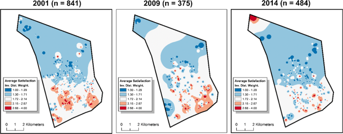
Inverse distance weighted (Inv. Dist. Weight) maps for each individual survey. The title of each panel corresponds to the year, and n corresponds to the number of surveys in each year. The color scheme is consistent across each year

Full size image

Reprints and Permissions

References

Allison P (2002) Missing data. Series in quantitative applications in the social sciences. Sage, Thousand Oaks, CA
Anselin L (1995) Local indicators of spatial association—LISA. Geogr Anal 27:93–115
Baruch Y, Holtom BC (2008) Survey response rate levels and trends in organizational research. Hum Rel 61:1139–1160
Bates D, Maechler M, Bolker B, Walker S (2015) Fitting linear mixed effects models using lme4. J Stat Softw 67:1–48
Bivand R, Piras G (2015) Comparing implementations of estimation methods for spatial econometrics. J Stat Softw 63:1–36
Bradford B, Stanko EA, Jackson J (2009) Using research to inform policy: the role of public attitude surveys in understanding public confidence and police contact. Polic J Pol Pract 3:139–148
Braga AA, Papachristos AV, Hureau DM (2012) The effects of hot spots policing on crime: an updated systematic review and meta-analysis. Justice Q 31:633–663
Brandl SG, Frank J, Worden RE, Bynum TS (1994) Global and specific attitudes toward the police: disentangling the relationship. Justice Q 11:119–134
Cao L (2015) Differentiating confidence in the police, trust in the police, and satisfaction with the police. Polic Int J Strat Manag 38:239–249
Christensen RHB (2015) Ordinal—regression models for ordinal data. R package version 2015.6-28. http://www.cran.r-project.org/package=ordinal/. Accessed 18 May 2018
Circo G, Melde C, McGarrell EF (2018) Fear, victimization, and community characteristics on citizen satisfaction with the police. Pol Int J Polic Strat Manag (ahead of print)
Cohen MA (2017) The social cost of a racially targeted police encounter. J Benefit Cost Anal 8:369–384
Correia ME (2010) Determinants of attitudes toward police of Latino immigrants and non-immigrants. J Crim Justice 38:99–107
Corsaro N, Frank J, Ozer M (2015) Perceptions of police practice, cynicism of police performance, and persistent neighborhood violence: an intersecting relationship. J Crim Justice 43:1–11
Curman AS, Andresen MA, Brantingham PJ (2014) Crime and place: a longitudinal examination of street segment patterns in Vancouver, BC. J Quant Criminol 31:127–147
Curtin R, Presser S, Singer E (2005) Changes in telephone survey nonresponse over the past quarter century. Pub Opin Q 69:87–98
Dillman DA (1978) Mail and telephone surveys: the total design method. Wiley, New York, NY
Ferdik FV, Wolfe SE, Blasco N (2014) Informal social controls, procedural justice and perceived police legitimacy: do social bonds influence evaluations of police legitimacy? Am J Crim Justice 39:471–492
Fotheringham AS, Brunsdon C, Charlton M (2003) Geographically weighted regression: the analysis of spatially varying relationships. Wiley, West Sussex
Gau JM (2015) Procedural justice, police legitimacy, and legal cynicism: a test for mediation effects. Pol Pract Res Int J 16:402–415
Gau JM, Corsaro N, Stewart EA, Brunson RK (2012) Examining macro-level impacts on procedural justice and police legitimacy. J Crim Justice 40:333–343
Graziano LM, Rosenbaum DP, Schuck AM (2014) Building group capacity for problem solving and police–community partnerships through survey feedback and training: a randomized control trial within Chicago’s community policing program. J Exp Criminol 10:79–103
Grott CJ, Albright J (2004) Billings police department crime and criminal justice survey. Washington State University, Pullman, WA
Grubesic TH (2008) Zip codes and spatial analysis: problems and prospects. Soc Econ Plan Sci 42:129–149
Haberman CP, Groff ER, Ratcliffe JH, Sorg ET (2015) Satisfaction with police in violent crime hot spots: using community surveys as a guide for selecting hot spots policing tactics. Crime Delinq 62:525–557
Higginson A, Mazerolle L (2014) Legitimacy policing of places: the impact on crime and disorder. J Exp Criminol 10:429–457
Hipp JR (2007) Block, tract, and levels of aggregation: neighborhood structure and crime and disorder as a case in point. Am Soc Rev 72:659–680
Hipp JR (2010) Resident perceptions of crime and disorder: how much is “Bias”, and how much is social environment differences? Criminology 48:475–508
Hipp JR, Boessen A (2013) Egohoods as waves washing across the city: a new measure of “neighborhoods”. Criminology 51:287–327
Hohl K, Bradford B, Stanko EA (2010) Influencing trust and confidence in the London metropolitan police results from an experiment testing the effect of leaflet drops on public opinion. Brit J Criminol 50:491–513
Kirk DS, Papachristos AV (2011) Cultural mechanisms and the persistence of neighborhood violence. Am J Soc 116:1190–1233
Klinger DA (1997) Negotiating order in patrol work: an ecological theory of police response to deviance. Criminology 35:277–306
Kochel TR (2011) Constructing hot spots policing: unexamined consequences for disadvantaged populations and for police legitimacy. Crim Just Pol Rev 22:350–374
Kochel TR (2018) Police legitimacy and resident cooperation in crime hotspots: effects of victimisation risk and collective efficacy. Pol Soc 28:251–270
Kochel TR, Weisburd D (2018) The impact of hot spots policing on collective efficacy: findings from a randomized field trial. Justice Q (online first)
Lai Y, Zhao JS (2010) The impact of race/ethnicity, neighborhood context, and police/citizen interaction on residents’ attitudes toward the police. J Crim Justice 38:685–692
Lai Y, Ren L, Greenleaf R (2017) Residence-based fear of crime: a routine activities approach. Int J Off Ther Comp Crimnol 61:1011–1037
Lee H, Vaughn MS, Lim H (2014) The impact of neighborhood crime levels on police use of force: an examination at micro and meso levels. J Crim Justice 42:491–499
Long JS (1997) Regression models for categorical and limited dependent variables. Sage, Thousand Oaks, CA
Lum C, Koper C, Telep C (2011) The evidence-based policing matrix. J Exp Criminol 7:3–26
Luo F, Ren L, Zhoa JS (2017) The effect of micro-level disorder incidents on public attitudes toward the police. Pol Int J Polic Strat Manag 40:395–409
Maguire ER, Johnson D (2010) Measuring public perceptions of the police. Pol Int J Polic Strat Manag 33:703–730
Mazerolle L, Antrobus E, Bennett S, Tyler TR (2013) Shaping citizen perceptions of police legitimacy: a randomized field trial of procedural justice. Criminology 51:33–63
Ratcliffe JH (2004) Geocoding crime and a first estimate of a minimum acceptable hit rate. Int J Geo Info Sci 18:61–72
Ratcliffe JH, Groff ER, Sorg ET, Haberman CP (2015) Citizens’ reactions to hot spots policing: impacts on perceptions of crime, disorder, safety and police. J Exp Criminol 11:393–417
Reisig MD, Correia ME (1997) Public evaluations of police performance: an analysis across three levels of policing. Pol Int J Strat Manag 20:311–325
Reisig MD, Parks RB (2000) Experience, quality of life, and neighborhood context: a hierarchical analysis of satisfaction with police. Justice Q 17:607–630
Rosenbaum DP, Schuck AM, Costello SK, Hawkins DF, Ring MK (2005) Attitudes toward the police: the effects of direct and vicarious experience. Police Q 8:343–365
Sampson RJ, Bartusch DJ (1998) Legal cynicism and (subcultural?) tolerance of deviance: the neighborhood context of racial differences. Law Soc Rev 32:777–804
Schuck AM, Rosenbaum DP (2005) Global and neighborhood attitudes toward the police: differentiation by race, ethnicity and type of contact. J Quant Criminol 21:391–418
Schuck AM, Rosenbaum DP, Hawkins DF (2008) The influence of race/ethnicity, social class, and neighborhood context on residents’ attitudes toward the police. Police Q 11:496–519
Silver E, Miller LL (2004) Sources of informal social control in Chicago neighborhoods. Criminology 42:551–584
Silver JR, Pickett JT (2015) Toward a better understanding of politicized policing attitudes: conflicted conservatism and support for police use of force. Criminology 53:650–676
Skogan WG (2005) Citizen satisfaction with police encounters. Police Q 8:298–321
Skogan WG (2006a) Asymmetry in the impact of encounters with police. Police Soc 16:99–126
Skogan WG (2006b) Police and community in chicago: a tale of three cities. Oxford University Press, New York, NY
Skogan WG (2009) Concern about crime and confidence in the police: reassurance or accountability? Police Q 12:301–318
Slocum TA, McMaster RB, Kessler FC, Howard HH (2005) Thematic cartography and geographic visualization, 2nd edn. Pearson, Upper Saddle River, NJ
Slocum LA, Taylor TJ, Brick BT, Esbensen FA (2010) Neighborhood structural characteristics, individual-level attitudes, and youths’ crime-reporting intentions. Criminology 48:1063–1100
Slovak JS (1986) Attachments in the nested community: evidence from a case study. Urban Aff Rev 21:575–597
Smith WR, Frazee SG, Davison EL (2000) Furthering the integration of routine activity and social disorganization theories: small units of analysis and the study of street robbery as a diffusion process. Criminology 38:489–524
Snijders T, Bosker R (2012) Multilevel analysis: an introduction to basic and advanced multilevel modeling. Sage, London
Solymosi R, Bowers K, Fujiyama T (2015) Mapping fear of crime as a context-dependent everyday experience that varies in space and time. Leg Criminol Psychol 20:193–211
Spelman W (2004) Optimal targeting of incivility-reduction strategies. J Quant Criminol 20:63–88
Steenbeek W, Weisburd D (2016) Where the action is in crime? An examination of variability of crime across different spatial units in the Hague, 2001–2009. J Quant Criminol 32:449–469
Sun IY, Triplett RA, Gainey RR (2004) Social disorganization, legitimacy of local institutions and neighborhood crime: an exploratory study of perceptions of the police and local government. J Crime Just 27:33–60
Sunshine J, Tyler TR (2003) The role of procedural justice and legitimacy in shaping public support for policing. Law Soc Rev 37:513–548
Taylor RB (1997) Social order and disorder of street blocks and neighborhoods: ecology, microecology, and the systemic model of social disorganization. J Res Crime Delin 34:113–155
Taylor RB, Lawton BA (2012) An integrated contextual model of confidence in local police. Police Q 15:414–445
Tyler TR (1990) Why people obey the law: procedural justice, legitimacy, and compliance. Yale University Press, New Haven, CT
Tyler TR, Jackson J (2014) Popular legitimacy and the exercise of legal authority: motivating compliance, cooperation, and engagement. Psychol Pub Policy Law 20:78–95
Van Craen M, Skogan WG (2015) Differences and similarities in the explanation of ethnic minority groups’ trust in the police. Eur J Crim 12:300–323
Webb VJ, Marshall CE (1995) The relative importance of race and ethnicity on citizen attitudes toward the police. Am J Police 14:45–66
Weisburd DL, Majmundar MK (2018) Proactive policing: effects on crime and communities. National Academies Press, Washington, DC
Weisburd DL, Telep CW (2014) Hot spots policing: what we know and what we need to know. J Cont Crim Just 30:200–220
Weisburd DL, Bushway SD, Lum C, Yang SM (2004) Trajectories of crime at places: a longitudinal study of street segments in the city of Seattle. Criminology 42:283–322
Weisburd DL, Hinkle J, Famega C, Ready J (2011) The possible “backfire” effects of hot spots policing: an experimental assessment of impacts on legitimacy, fear and collective efficacy. J Exp Criminol 7:297–320
Weisburd DL, Groff ER, Yang SM (2012) The criminology of place: street segments and our understanding of the crime problem. Oxford University Press, New York, NY
Weisburd DL, Telep CW, Lawton BA (2014) Could innovations in policing have contributed to the New York City crime drop even in a period of declining police strength?: the case of stop, question and frisk as a hot spots policing strategy. Justice Q 31:129–153
Weitzer R, Tuch SA (2005) Determinants of public satisfaction with the police. Police Q 8:279–297
Wells W, Schafer JA, Varano SP, Bynum TS (2006) Neighborhood residents’ production of order: the effects of collective efficacy on responses to neighborhood problems. Crime Delinq 52:523–550
Wheeler AP, Worden RE, McLean SJ (2016) Replicating group-based trajectory models of crime at micro-places in Albany, NY. J Quant Criminol 32:589–612
Wolfe SE, Nix J, Kaminski R, Rojek J (2016) Is the effect of procedural justice on police legitimacy invariant? Testing the generality of procedural justice and competing antecedents of legitimacy. J Quant Criminol 32:253–282
Worden RE, McLean SJ (2017) Mirage of police reform: procedural justice and police legitimacy. University of California Press, Oakland, CA
Wu Y, Sun IY, Triplett RA (2009) Race, class or neighborhood context: which matters more in measuring satisfaction with police? Justice Q 26:125–156
Zahnow R, Mazerolle L, Wickes R, Corcoran J (2017) Living near violence: how proximity to violence shapes perceptions of police effectiveness and confidence in police. J Environ Psychol 53:138–144
Zhao JS, Tsai C, Ren L, Lai Y (2014) Public satisfaction with police control of disorder crime: does the public hold police accountable? Justice Q 31:394–420
Zhao JS, Lawton B, Longmire D (2015) An examination of the micro-level crime-fear of crime link. Crime Delinq 61:19–44
Acknowledgements