Assessing Categorical Effects in Machine Learning Models

One model diagnostic for machine learning models I like are accumulated local effects (ALE), see Wheeler & Steenbeek (2021) for an example and Molnar (2020) for a canonical mathematical reference. With these we get some ex-ante interpretability of models – I use this for mostly EDA of the final fitted model. Here is an example of seeing the diffusion effect of DART stations on robberies in Dallas from my cited paper:

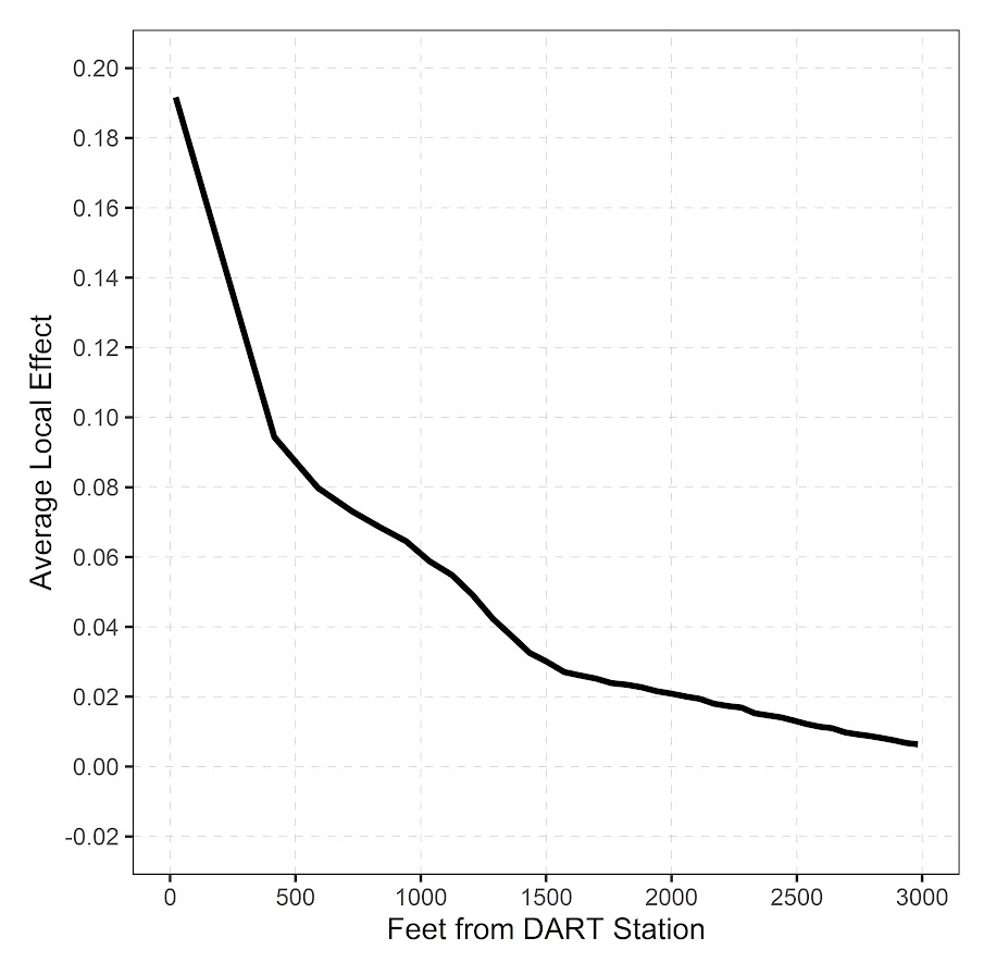
So the model is behaving as expected – nearby DART stations causes an uptick, and that slowly diffuses away. And the way the ML model is set up it can estimate that diffusion effect, I did not apriori specify what that should look like.

These are essentially average/marginal effects (or approximate derivatives) for complicated machine learning models. In short pseudoish/python code, pretend we have a set of data D and a model, the local effect of variable x at the value 5 is something like:

D['x'] = 5 # set all the data for x to value 5
pred5 = mod.predict(D)
D['x'] = 5 + 0.001 # change value x by just alittle
predc = mod.predict(D)
loc_eff = (pred5 - predc)/0.001
print(loc_eff.mean())

So in shorthand [p(y|x) - p(y|x+s)]/s, so s is some small change (approximate the continuous derivative via finite differences). Then you generate these effects (over your sample), for various values of x, and then make a plot.

Many people say that this only applies to numerical features. So say we have a categorical effect with three variables, a/b/c. We could calculate p(y|a) and p(y|b), but because a - b is not defined (what is the difference in categorical variables), we cannot have anything like a derivative in the ALE for categorical features.

This seems to me though short sited. While we cannot approximate a derivative, the value p(y|a) - p(y|b) is pretty interpretable without the division – this is the predicted difference if we switch from category a to category b. Here I think a decent default is to simply do p(y|cat) - mean(p(y|other cat)), and then you can generate average categorical effects for each category (with very similar interpretation to ALEs). For those who know about regression contrasts, this would be like saying we have dummy variables for A/B/C, and the effect of A is contrast coded via 1,-1/2,-1/2.

Here is a simple example in python. For data see my prior post on the NIJ recidivism challenge or mine and Gio’s working paper (Circo & Wheeler, 2021). Front end cleaning up the data is very similar. I use a catboost model here.

import catboost
import numpy as np
import pandas as pd

# Ommitted Code, see 
# https://andrewpwheeler.com/2021/07/24/variance-of-leaderboard-metrics-for-competitions/
# for how pdata is generated
pdata = prep_data(full_data)

# Original train/test split
train = pdata[pdata['Training_Sample'] == 1].copy()
test = pdata[pdata['Training_Sample'] == 0].copy()

# estimate model, treat all variables as categorical
y_var = 'Recidivism_Arrest_Year1'
x_vars = list(pdata)
x_vars.remove(y_var)
x_vars.remove('Training_Sample')
cat_vars = list( set(x_vars) - set(more_clip) )

cb = catboost.CatBoostClassifier(cat_features=cat_vars)
cb.fit(train[x_vars],train[y_var])

Now we can do the hypothetical change the category and see how it impacts the predicted probabilities (you may prefer to do this on the logit scale, but since it is conditional on all other covariates it should be OK IMO). Here I calculate the probabilities over each of the individual PUMAs in the sample.

# Get the differences in probabilities swapping
# out each county, conditional on other factors
pc = train.copy()
counties = pd.unique(train['Residence_PUMA']).tolist()
res_vals = []
for c in counties:
    pc['Residence_PUMA'] = c
    pp = cb.predict_proba(pc[x_vars])[:,1]
    res_vals.append(pd.Series(pp))

res_pd = pd.concat(res_vals,axis=1)
res_pd.columns = counties
res_pd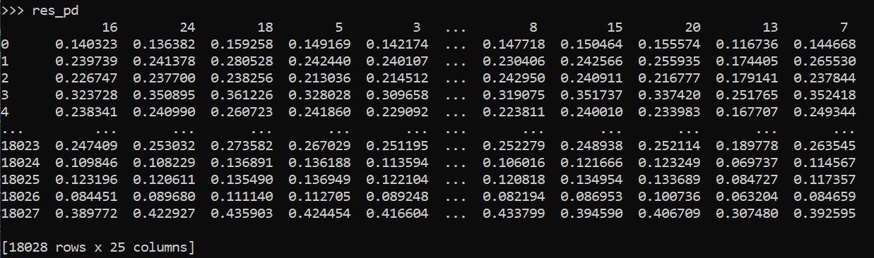

So you can see for the person in the first row, if they were in PUMA 16, they would have a predicted probability of recidivism of 0.140. If you switched them to PUMA 24, it changes to 0.136. So you can see the PUMA overall doesn’t appear to have much of an impact on the recidivism prediction in this catboost model.

Now here is leave one out centering as I stated before. So we compare PUMA 16 to the average of all other PUMAs, within each row.

# Now mean center
n = res_pd.shape[1]
row_sum = res_pd.sum(axis=1)
row_adj = (-1*res_pd).add(row_sum,axis=0)/(n-1)
ycent = res_pd - row_adj
ycent

And now we can do various column aggregations to get the average categorical effects per each category. You can do whatever aggregation you want (means/medians/percentiles). (I’ve debated on making my own library to make ALEs a bit more general and return variance estimates as well.)

# Now can get mean/sd/ptils
mn = ycent.mean(axis=0)
sd = ycent.std(axis=0)
low = ycent.quantile(0.025,axis=0)
hig = ycent.quantile(0.975,axis=0)
fin_stats = pd.concat([mn,sd,low,hig],axis=1)
# Cleaning up the data
fin_stats.columns = ['Mean','Std','Low','High']
fin_stats.reset_index(inplace=True)
fin_stats.rename(columns={"index":"PUMA"}, inplace=True)
fin_stats.sort_values(by='Mean',ascending=False,
                      inplace=True,ignore_index=True)
fin_stats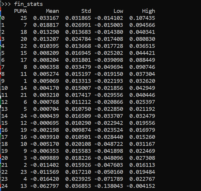

And we can see that while I sorted the PUMAs and PUMA 25 has a mean effect of 0.03, its standard deviation is quite high. The only PUMA that the percentiles do not cover 0 is PUMA 13, with a negative effect of -0.06.

Like I said, I like these more so for model checking/EDA/face validity. Here I would dig into further PUMA 25/13, make sure nothing funny is going on with the data (and whether I should try to tease out more features from these in real life if I had access to the source data, e.g. smaller aggregations). The other PUMAs though are quite unremarkable and have spreads of +/-2 percentage points pretty consistently.

References

• Circo, G., & Wheeler, A.P. (2021). National Institute of Justice Recidivism Forecasting Challange Team “MCHawks” Performance Analysis. CrimRXiv.
• Molnar, C. (2020). Interpretable machine learning. Ebook.
• Wheeler, A. P., & Steenbeek, W. (2021). Mapping the risk terrain for crime using machine learning. Journal of Quantitative Criminology, 37(2), 445-480.