

Blog | Electric Field Due To A System Of Charges | MATLAB Helper ®
source link: https://matlabhelper.com/blog/matlab/electric-field-due-to-a-system-of-charges/
Go to the source link to view the article. You can view the picture content, updated content and better typesetting reading experience. If the link is broken, please click the button below to view the snapshot at that time.

Electric field due to a system of charges
June 10, 2022
By Anuradha Viswanathan
Need Urgent Help?
Our experts assist in all MATLAB & Simulink fields with communication options from live sessions to offline work.
testimonials
Philippa E. / PhD Fellow
I STRONGLY recommend MATLAB Helper to EVERYONE interested in doing a successful project & research work! MATLAB Helper has completely surpassed my expectations. Just book their service and forget all your worries.
Yogesh Mangal / Graduate Trainee
MATLAB Helper provide training and internship in MATLAB. It covers many topics of MATLAB. I have received my training from MATLAB Helper with the best experience. It also provide many webinar which is helpful to learning in MATLAB.
The electric field is a significant quantity when dealing with problems in electromagnetism and has several applications in various disciplines. The study of electric fields due to static charges is a branch of electromagnetism – electrostatics. There are several applications of electrostatics, such as the Van de Graaf generator, xerography, and laser printers. Every charged object creates a field in the space surrounding it. Michael Faraday was known for his discovery of electromagnetic induction and the introduction of the concept of fields in the 19th century. His vision laid the foundation for many discoveries in modern electromagnetic theory. An electric field is carried by subatomic particles, namely, the proton carrying a positive charge and the electron carrying a negative charge. Along with neutrons, these particles make up all the atoms in the universe. Therefore it is essential to study the visual and quantitative relationships between electric fields and equipotential lines.
Electrostatic force and electric field
When a charge is in the vicinity of another charge, it experiences a force exerted by the neighboring charge. By Coulomb’s law, the forces of attraction or repulsion exerted between two point charges varies in direct proportion to the product of the magnitude of the charges and vary inversely as the square of the distance between them. This law is analogous to Newton’s law of universal gravitation. The differences are that electric fields are much stronger than the gravitational field and electric forces arising from the electric fields are either attractive or repulsive depending on the sign of the charges. The electric field is defined by the force exerted by a point charge on a unit test charge and is given by force per unit charge. Just as the gravitational force arises from a gravitational field, the electric force arises from the electric field. These are given by the formulae,

where,
r – the distance between the source charge and test charge
Q – source charge
q – test charge

and the electric field is given by,


Figure 1: Electric field lines - positive point charge
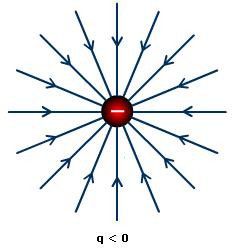
Figure 2: Electric field lines - negative point charge
Every point in the 3D space is subject to the electric field, and the field around a point charge is spherically symmetric. For any given location, the electric field can be represented by arrows that change in length in proportion to the strength of the electric field. This is known as the vector field map which has the magnitude and direction of the electric field at evenly spaced points on a grid, and this is the representation created with the MATLAB code using the quiver plot. However in reality, it is more convenient to represent electric fields with patterns of electric field lines rather than with arrows. These field lines are created by connecting the field vectors together. These patterns of field lines extend from infinity to the source charge. The electric field lines originate from a positive charge, terminate at a negative charge, and never intersect. These field lines are directed radially outward for positive and inward for negative charges.

Figure 3: Electric field lines and equipotential lines-Equal and opposite charges
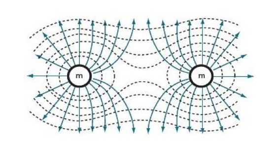
Figure 4: Electric field and equipotential lines - equal positive charges
The electric field does not depend on the test charge and depends only on the distance from the source charge to the test charge and the source charge. Extending this idea to a system of charges, the combined electric field due to these charges turns out as the vector sum of the individual charges, which is given by the superposition principle as,

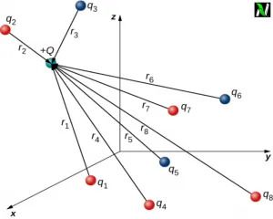
Figure 5: Superposition principle for multiple point charges
Relationship between electric field lines and equipotential lines
There are lines along which the electric potential is equal, and these can be visualized as contour lines/isolines surrounding the charge. These are known as the equipotential lines, and as the name suggests, the electric potentials are the same everywhere along these lines or equipotential surfaces(in 3D). The equipotential lines are analogous to the contour lines on a topographical map that indicates lines of equal elevation and hence equal gravitational potential energy.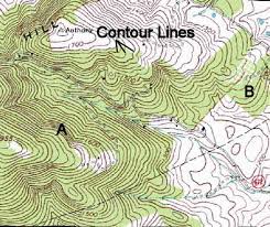
Figure 6: Topographical Map - Contour lines
So the work done by the gravitational field would be zero as you walk along the contour lines of constant elevation. The equipotential lines are along a direction that is perpendicular to the electric field and the electric potential is a scalar quantity. Thus electric field lines are pointed in a direction towards maximum potential decrease. If we take a test charge in an electric field and move it against the electric field, there is a resulting work done to move it in that direction. However, moving the test charge along an equipotential line results in no change in the potential energy, which implies that the electric field does no work in moving the charge along this line(since the direction of the electric force is perpendicular to the direction of motion). The equipotential lines closer to the source would be more closely spaced owing to a stronger electric field at those locations and would become more widely spaced at distances further away from the source. These phenomena can be explained by observing that the test charge placed at an initial potential would accelerate and hence gain kinetic energy in a direction along the electric field lines very quickly. This would result in reaching a line of lower potential energy at a very small distance from the initial position. At points of a weaker electric field, it would accelerate away slower and travel a longer distance before losing potential energy and gaining kinetic energy.
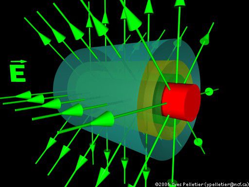
Figure 7: Equipotential surfaces and electric field lines- Cylinder
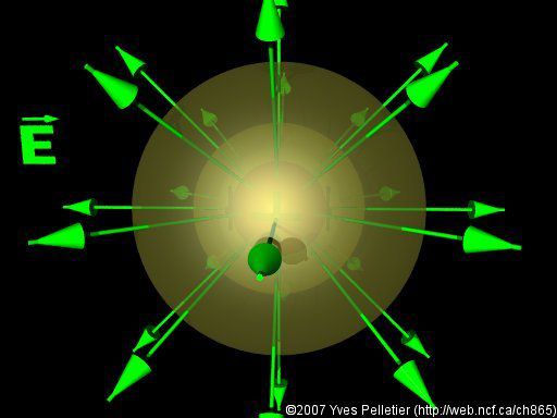
Figure 8: Equipotential surfaces and electric field lines- Sphere
Now that we have seen the visual relationship let us look at the quantitative relationship between the electric field, potential energy, and electric potential.
A test charge that moves along the direction of the electric field would experience an electrostatic force of


And the work done by the force to move it along displacement ‘dx’ is given by

Therefore the change in potential energy is the negative of the work done since it moves in the direction of the field lines

The electric potential difference or the voltage is defined as the electric potential energy per unit charge and given by,

Without the assumption of uniformity of the electric field, it can be expressed as the gradient of the potential in the direction of x as,

and hence

Equipotential lines and field lines for a system of charges
i. Equal positive charges
Consider a system of two equal positive charges, as shown in Figure 4. As described earlier, the electric field lines would point away from each other due to electrostatic repulsion. The dotted lines in Figure 4 represent the equipotential lines.
And since the equipotential surfaces are perpendicular to the field lines, they change from the spherical surface and take an egg-shaped form. They appear to merge as you go further away from the charges. At a distance much bigger than the separating distance between the charges, the equipotential surface around the two charges becomes spherical.
ii. Unequal positive charges
For the case of unequal positive charges, the only difference from the prior case is that the size of the spherical surface of the individual charge increases in proportion to the magnitude of the charge and forms a larger spherical equipotential surface around the charge
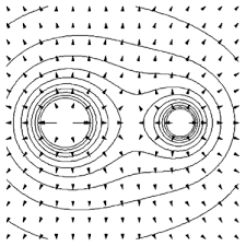
Figure 9 : Equipotential lines and electric field - unequal positive charges
iii. Equal negative charges
For the case of two negative charges, the equipotential is the same as for the case of two positive charges.
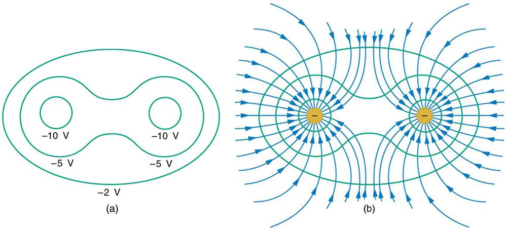
Figure 10: Equipotential lines and electric field - equal negative charges
iv. Equal and opposite charges - Dipole
A dipole consists of two charges of equal and opposite signs separated by a distance. Taking the case of a dipole, the electric field lines terminate on the negative charge and emerge from the positive charge. Therefore, to maintain perpendicularity with the field lines, the equipotential lines flatten out at the centre of the two charges and would never merge, forming a sheet/line of zero potential. This is as seen in Figure 3, with the red dashed lines being the equipotential lines.
For unequal and opposite charges, the equipotential surface of the larger positive/negative charge dominates over the smaller charge. At distances sufficiently far from the charges would appear to merge with each other, forming surfaces of positive/negative potential, and the system of charges would appear as a single positive/negative charge, as shown in the figure below.
Figure 11: Electric field lines- unequal and opposite charges
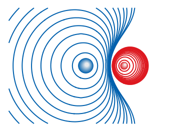
Figure 12: Equipotential lines - unequal and opposite charges
Thus the net effect of a system of charges can be extended to any number of charges, and the field lines and equipotential surfaces are formed according to the above-stated principles.
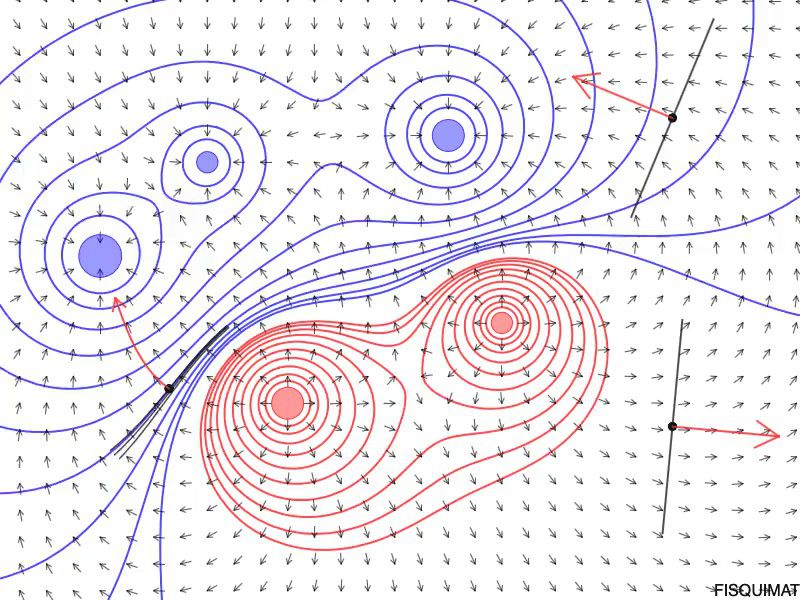
Figure 13: Equipotential lines and electric field - a system of charges
MATLAB Code implementation
Get Access to
Code & Report!
The theory of electric fields in static equilibrium is electrostatics. Learn about electric fields and equipotential lines due to a generalized system of charges with the visualization and quantitative relationships using MATLAB; Developed in MATLAB R2022a
% the electric field and equipotential surfaces in 2D along with
% surface-contour plot of voltage
% Topic: Electric field and potential due to a system of charges
% Website: https://matlabhelper.com
% Date: 25-04-2022
clear;
close all;
% The constant is calculated taking the charges to be in the order of nano
% coulombs and the relative permittivity as one. This would give the resulting
% constant as 9.
% Charges in the order of nano- coulombs
Q = [4,-1, -4, 1, 3, -2, -5];
% Array of locations
X = [-10,-5,5,10,10,15,15];
Y = [0,5,10,5,10,10,20];
% Number of charges
n = length(Q);
Outputs
i. Charges : [ 1, 1]
Charge locations : X = [-5,5]; Y = [0,5];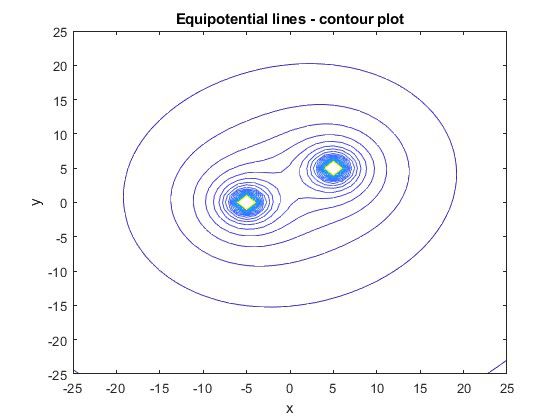
Figure 14 : Equipotential lines - contour plot
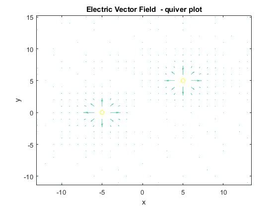
Figure 15: Electric Vector field - quiver plot
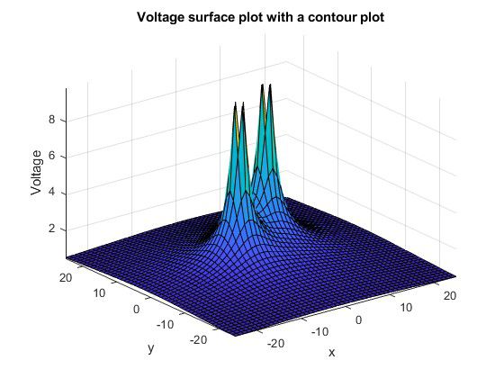
Figure 16: Voltage - surface plot with contour plot
ii. Charges : [ -1, -1]
Charge locations : X = [-5,5]; Y = [0,5];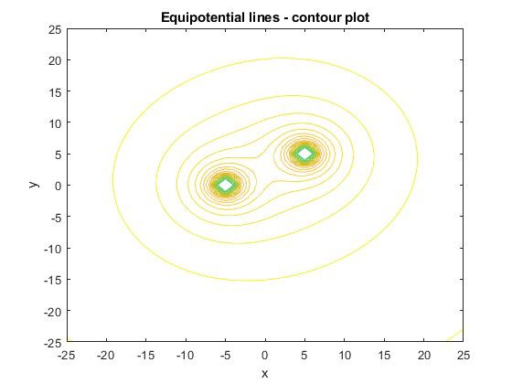
Figure 17: Equipotential lines - contour plot
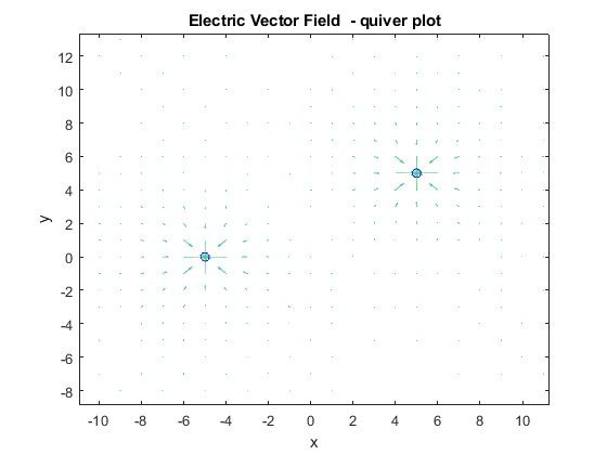
Figure 18: Electric Vector field - quiver plot
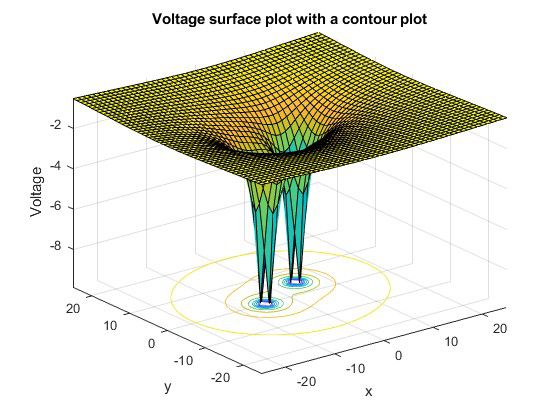
Figure 19: Voltage - surface plot with contour plot
iii. Charges : [4,1, -4, -1];
Charge locations : X = [-10,-5,5,10]; Y = [0,5,10,5];
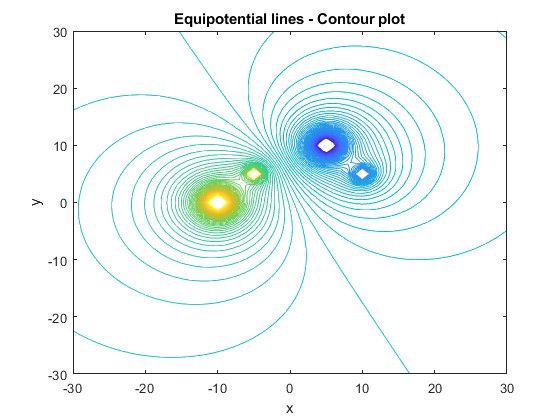
Figure 20: Equipotential lines - contour plot
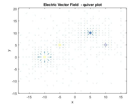
Figure 21: Electric Vector field - quiver plot
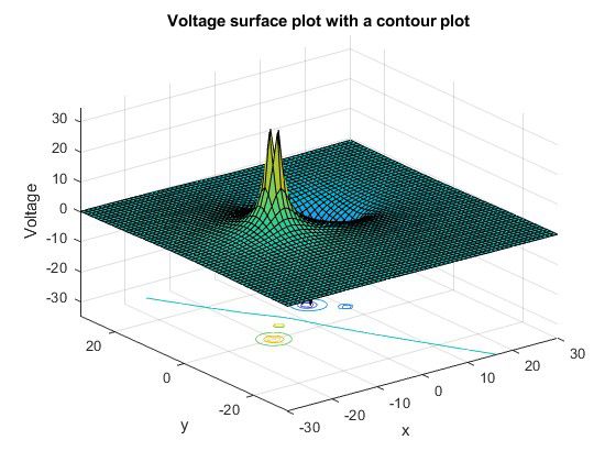
Figure 22: Voltage - surface plot with contour plot
v. Charges : [4,-1, -4, 1, 3, -2, -5];
X = [-10,-5,5,10,10,15,15]; Y = [0,5,10,5,10,10,20];
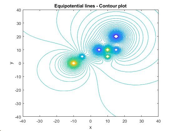
Figure 23: Equipotential lines - contour plot
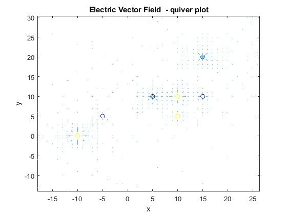
Figure 24: Electric Vector field - quiver plot
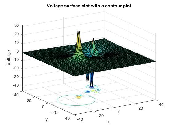
Figure 25: Voltage - surface plot with contour plot
Conclusion
The visualization and computation of the electric fields, equipotential lines and voltage have been described in the above sections using MATLAB. The relationship between electric fields and equipotential surfaces has been discussed for various charge combinations, and the corresponding code results have been generated for a system of charges. It builds the concept from a system of two charges and extends it to multiple charges.
Did you find some helpful content from our video or article and now looking for its code, model, or application? You can purchase the specific Title, if available, and instantly get the download link.
Thank you for reading this blog. Do share this blog if you found it helpful. If you have any queries, post them in the comments or contact us by emailing your questions to [email protected]. Follow us on LinkedIn Facebook, and Subscribe to our YouTube Channel. If you find any bug or error on this or any other page on our website, please inform us & we will correct it.
If you are looking for free help, you can post your comment below & wait for any community member to respond, which is not guaranteed. You can book Expert Help, a paid service, and get assistance in your requirement. If your timeline allows, we recommend you book the Research Assistance plan. If you want to get trained in MATLAB or Simulink, you may join one of our training modules.
If you are ready for the paid service, share your requirement with necessary attachments & inform us about any Service preference along with the timeline. Once evaluated, we will revert to you with more details and the next suggested step.
Education is our future. MATLAB is our feature. Happy MATLABing!
About the author
Anuradha Viswanathan
MATLAB Developer at MATLAB Helper,
M.S in Telecommunications and Networking,
M.S in Physics
</div
Recommend
About Joyk
Aggregate valuable and interesting links.
Joyk means Joy of geeK