

Python Code of Mini-Batch Gradient Descent
source link: https://capallen.gitee.io/2018/Python%20code%20for%20mini%20batch%20gradient%20descent.html
Go to the source link to view the article. You can view the picture content, updated content and better typesetting reading experience. If the link is broken, please click the button below to view the snapshot at that time.
Python Code of Mini-Batch Gradient Descent
Mini-Batch Gradient Descent是介于batch gradient descent(BGD)和stochastic gradient descent(SGD)之间的一种线性回归优化算法,它是将数据分为多个小的数据集(batches),每个数据集具有大致相同的点数,然后在每个数据集中应用Absolute Trick或者是Square Trick算法,来更新回归系数。
它的运算速度比BSD快,比SGD慢;精度比BSD低,比SGD高。
import numpy as np
import matplotlib.pyplot as plt

np.random.seed(42)

def MSEStep(X, y, W, b, learn_rate = 0.001):
    """
    This function implements the gradient descent step for squared error as a
    performance metric.

Parameters
    X : array of predictor features
    y : array of outcome values
    W : predictor feature coefficients
    b : regression function intercept
    learn_rate : learning rate

Returns
    W_new : predictor feature coefficients following gradient descent step
    b_new : intercept following gradient descent step
    """

# compute errors
    # the squared trick formula
    y_pred = np.matmul(X, W) + b #Attention:the order of X and W
    error = y - y_pred
    #y_pred is a 1-D array,so is the error

# compute steps
    W_new = W + learn_rate * np.matmul(error, X) #Attention:the order of X and error
    b_new = b + learn_rate * error.sum()
    return (W_new, b_new)

def miniBatchGD(X, y, batch_size = 20, learn_rate = 0.005, num_iter = 25):
    """
    This function performs mini-batch gradient descent on a given dataset.

Parameters
    X : array of predictor features
    y : array of outcome values
    batch_size : how many data points will be sampled for each iteration
    learn_rate : learning rate
    num_iter : number of batches used

Returns
    regression_coef : array of slopes and intercepts generated by gradient
      descent procedure
    """
    n_points = X.shape[0]
    W = np.zeros(X.shape[1]) # coefficients
    b = 0 # intercept

# run iterations
    #hstack为水平堆叠函数 为什么要堆叠呢?
    #类似zip,可以实现for W,b in regression_coef:print W,b来提取W和b
    regression_coef = [np.hstack((W,b))]
    for _ in range(num_iter):
        #从0-100中随机选择batch_size个数,作为batch
        batch = np.random.choice(range(n_points), batch_size)
        #按照batch从X中选出数据
        X_batch = X[batch,:]#为2-D矩阵
        y_batch = y[batch]#为1-D数组
        W, b = MSEStep(X_batch, y_batch, W, b, learn_rate)
        regression_coef.append(np.hstack((W,b)))

return (regression_coef)

if __name__ == "__main__":
    # perform gradient descent
    data = np.loadtxt('data.csv', delimiter = ',')
    X = data[:,:-1]#提取第一列,为2-D矩阵
    y = data[:,-1]#提取第二列,为1-D数组
    regression_coef = miniBatchGD(X, y)

# plot the results
    plt.figure()
    X_min = X.min()
    X_max = X.max()
    counter = len(regression_coef)
    for W, b in regression_coef:
        counter -= 1
         #color为[R,G,B]的列表,范围都在0-1之间,[0,0,0]为黑色,[1,1,1]为白色
        color = [1 - 0.92 ** counter for _ in range(3)]
        #绘制一条点(X_min,X_min * W + b)与点(X_max, X_max * W + b)之间的一条直线
        plt.plot([X_min, X_max],[X_min * W + b, X_max * W + b], color = color)
    plt.scatter(X, y, zorder = 3)
    plt.show()
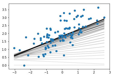
在结果中,颜色最浅的是最开始的回归线,最深的则为最终的回归线。
理论知识参见Linear Regression 总结,这里只对代码中出现的新函数或新用法进行讲解。
numpy.matmul(a,b)
该函数用来计算两个arrays的乘积。
需要注意的是,由于a和b维度的不同,会使得函数的结果计算方式不同,一共三种:
如果a和b都是2维的,则做普通矩阵乘法
a = [[1, 0], [0, 1]]
b = [[4, 1], [2, 2]]
np.matmul(a, b)
out:
array([[4, 1],
[2, 2]])如果a和b中有一个是大于2维的,则会将其理解为多个矩阵stack后的结果,进行计算时也会进行相应的拆分运算
a = np.arange(2*2*4).reshape((2,2,4))
b = np.arange(2*2*4).reshape((2,4,2))
np.matmul(a,b).shape
out:
(2, 2, 2)a被理解为2个2x4矩阵的stack
array([[[ 0,  1,  2,  3],
        [ 4,  5,  6,  7]],

[[ 8,  9, 10, 11],
        [12, 13, 14, 15]]])
b被理解为2个4x2矩阵的stack
array([[[ 0,  1],
        [ 2,  3],
        [ 4,  5],
        [ 6,  7]],

[[ 8,  9],
        [10, 11],
        [12, 13],
[14, 15]]])np.matmul(a,b)会将a中的两个矩阵与b中的两个矩阵对应相乘,每对相乘的结果都是一个2x2的矩阵,所以结果就是一个2x2x2的矩阵。如果a或b有一个是一维的,那么就会为该一维数组补充1列或1行,进而提升为二维矩阵,然后用非补充行或列去和另外一个二维矩阵进行运算,得到的结果再将补充的1去掉。(这个是最难理解的,可以多测试下,用代码结果理解)
a = [[1, 0], [0, 1]]
b = [1, 2]
np.matmul(a, b)
out:
array([1, 2])a是一个2x2的矩阵,b是一个shape为(2,)的一维数组,那么matmul的计算步骤如下:
- 计算中,矩阵a在前,数组b在后,所以需要让a的列数与升维之后b矩阵的行数相等
- 所以,升维后b矩阵的shape应为(2,1),这个1添加到了列上
- 进行矩阵乘法计算,得到shape为(2,1),这时候再将这个1去掉
- 最终结果的shape为(2,),变为一维数组
我们试着将a与b的顺序对调,看一下matmul是怎么计算的:
- 对调后,数组b在前,矩阵a在后,需要将升维后b矩阵的列数与矩阵a的行数相等
- 所以,升维后b矩阵的shape应该为(1,2),这个1添加到了行上
- 进行矩阵乘法,得到的shape为(1,2),将这个1去掉
- 最终结果的shape为(2,),变为一维数组
numpy.hstack()
我们先来看看numpy.stack()函数。
- 函数用法为:numpy.stack(arrays,axis = 0)
- 第一个参数为arrays,可以输入多维数组或者列表,也可以输入由多个一维数组或列表组成的元组
- 第二个参数为axis,输入数字,决定了按照arrays的哪个维度进行stack。比如说,输入的arrays的shape为(3,4,3),那么axis = 0/1/2就分别对应arrays的组/行/列。
这个函数中的axis有些抽象,我们看具体示例:
- 定义了一个列表
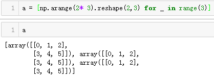
结果的排版有点问题,为了方便后面对照,把结果对齐如下:
[
    array([[0,1,2],[3,4,5]]),
    array([[0,1,2],[3,4,5]]),
    array([[0,1,2],[3,4,5]])
]
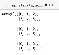
axis = 0,则按照第0个维度
组进行堆叠,即: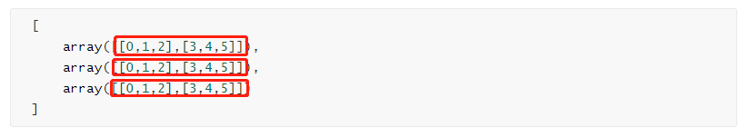
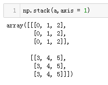
axis = 1,则按照第1个维度
行进行堆叠,即: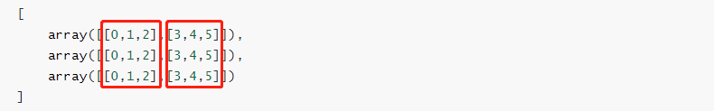
axis = 2,则按照第二个维度
列进行堆叠,即: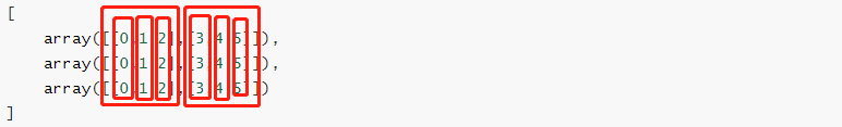
这个基本很少用到。
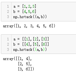
**numpy.hstack()**函数就是horizontal(水平)方向的堆叠,示例:
**numpy.vstack()**函数就是在垂直方向堆叠。
ndarray的切片
一维ndarray的切片方式和list无异,这里主要讲一下二维矩阵的切片方法。
a = np.arange(4*4).reshape(4,4)
print(a)
out:
array([[ 0,  1,  2,  3],
       [ 4,  5,  6,  7],
       [ 8,  9, 10, 11],
       [12, 13, 14, 15]])
a[:,:-1]
out:
array([[ 0,  1,  2],
       [ 4,  5,  6],
       [ 8,  9, 10],
       [12, 13, 14]])
这里可以看出,我们筛选了a矩阵中前三列的所有行,这是如何实现的呢?
切片的第一个元素:表示的是选择所有行,第二个元素:-1表示的是从第0列至最后一列(不包含),所以结果如上所示。
再看一个例子:
a[1:3,:]
out:
array([[ 4,  5,  6,  7],
       [ 8,  9, 10, 11]])
筛选的是第2-3行的所有列。
- 一个常用的切片
以列的形式获取最后一列数据:
a[:,3:]
out:
array([[ 3],
       [ 7],
       [11],
       [15]])
以一维数组的形式获取最后一列数据:
a[:,-1]
out:
array([ 3,  7, 11, 15])
上面两种方法经常会用到,前者的shape为(4,1),后者为(4,)。
matplotlib相关
color
代码中涉及到的语句为:
color = [1 - 0.92 ** counter for _ in range(3)]
matplotlib中的color可以输入RGB格式,即[R,G,B],这里值得注意的是它们的取值范围都在0到1之间,其中[0,0,0]为黑色,[1,1,1]为白色。
在如上语句中,列表由三个相等的数值元素组成,保证了颜色为白-灰-黑,数值随着counter的减小,由1趋近于0,反映在可视化上就是颜色由白逐渐变黑。
这真是一个画渐变过程的好方法呀!!!
plot([x_1,x_2],[y_1,y_2])
这里就是两点式绘图,根据点(x_1,y_1)和点(x_2,y_2)画一条直线。
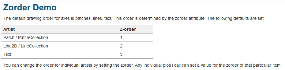
zorder
也就是z-order,类似于PS里面的图层顺序,下面的图层会被上面的图层遮挡。
参考Zorder Demo中队zorder的介绍,可以知道,zorder越大,图层越靠上,所以在上面的代码中,我们在scatter中设定zorder为3,也就是最上层,这样就可以保证渐变的回归线不会压在散点图上面了。
Recommend
About Joyk
Aggregate valuable and interesting links.
Joyk means Joy of geeK