Cointegration analysis of Ethereum and BitCoin

So a friend recently has heavily encouraged investment into Ethereum and NFTs. Part of the motivation of these cryptocurrencies is to be independent of fiat currency. So that lends itself to a hypothesis – are cryptocurrency prices and more typical securities independent? Or are we simply seeing similar trends in these different securities over time? This is a job for cointegration analysis. The python code is simple enough to follow along in a blog post.

So first I import the libraries I am using – it leverages the Yahoo finance API to download ticker data (here I analyze closing prices), and statsmodels to conduct the various analyses in python.

from datetime import datetime
import numpy as np
import pandas as pd
import yfinance as yf
import matplotlib.pyplot as plt

from statsmodels.tsa.stattools import adfuller, ccf
from statsmodels.tsa.api import VAR
from statsmodels.tsa.vector_ar import vecm

Now we can download the ticker data, here I will analyze BitCoin and Ethereum, along with Gold prices and the S&P 500 index fund.

# BTC-USD : Bitcoin
# ETH-USD : Ethereum
# ^GSPC ; S&P 500
# GC=F : Gold

end_date = datetime.now().strftime("%Y-%m-%d")
print(end_date) #running as of 2/9/2022

tick_str = 'BTC-USD ETH-USD ^GSPC GC=F'
dat = yf.download(tick_str,start='2017-01-01',end=end_date)

Now for data prep – I am going to interpolate missing data (for when the market was closed). Then I only subset out Fridays at close to conduct a weekly analysis. Even weekly is too short for me to bother with rebalancing if I do decide to invest.

# Fill in missing data before sub-sampling to once a week
dat2 = dat.interpolate()

# Only Fridays close post 11/9/2017
dat2.reset_index(inplace=True)
after = pd.to_datetime('2017-11-09')
sel = (dat2.Date >= after) & (dat2.Date.dt.weekday == 4) #Friday
sdat = dat2.loc[sel,['Date','Close']]
sdat.columns = ['Date'] + ['BitCoin','Eth','S&P 500','Gold']
sdat.set_index('Date',inplace=True)

Now lets look at the overall trends by superimposing these four stocks on the same graph. Just min-max normalizing to range from 0 to 1.

# Time Series Graphs of Each
# Normalized to be 0/1
snorm = sdat.copy()
for v in sdat:
    mi,ma = sdat[v].min(),sdat[v].max()
    snorm[v] = (sdat[v] - mi)/(ma-mi)

# All four series on the same graph
snorm.plot(linewidth=2)
plt.show()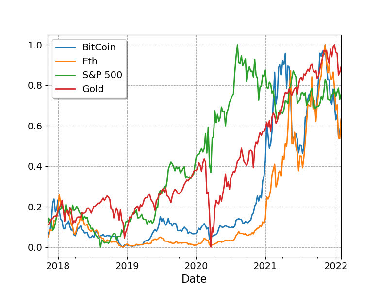

So you can see these all appear to follow a similar upward trajectory after Covid hit in 2020, although crypto has way more volatility recently. If we subset out just the crypto’s, we can see how they trend with each other more easily.

s2 = sdat.copy()
s2['BitCoin/10'] = s2['BitCoin']/10
s2[['BitCoin/10','Eth']].plot(linewidth=2)
plt.show()

So based on this, I would say that maybe Bitcoin is a leading indicator of Ethereum (increases in BitCoin precede increases in Eth with maybe just a week lag).

Typically with any time series analysis like this, we are concerned with whether the series are stationary. Just going off of my Ender’s Applied Econometric Time Series book, we typically look at the Adjusted Dickey-Fuller test for the levels:

# Integration analysis
adfuller(sdat['BitCoin'], regression='ct', maxlag=5, autolag='t-stat', regresults=True)

And we can see this fails to reject the null, so we would conclude the series is integrated. Since we have a fairly large sample here (over 200 weeks), the test should be reasonably powered. If we then take the first differences and conduct the same test, we then reject the null of an integrated series (here for Bitcoin).

# Create differenced data
sdiff = sdat.diff().dropna()

# All appear 1st order integrated!
adfuller(sdiff['BitCoin'], regression='ct', maxlag=5, autolag='t-stat', regresults=True)

So this reasonably suggests Bitcoin is an I(1) process. Doing the same for all of the other securities in this example you come to the same inference, all integrated of order 1 (which is very typical for stock data).

Using the differenced data, we can see the cross-correlations between different securities. In this example, it appears BitCoin/Ethereum just have a large 1 positive lag, and close to 0 after that.

# Only 1 lag positive in differenced data
pd.Series(ccf(sdiff['BitCoin'],sdiff['Eth'])[:10]).plot(kind='bar',grid=False)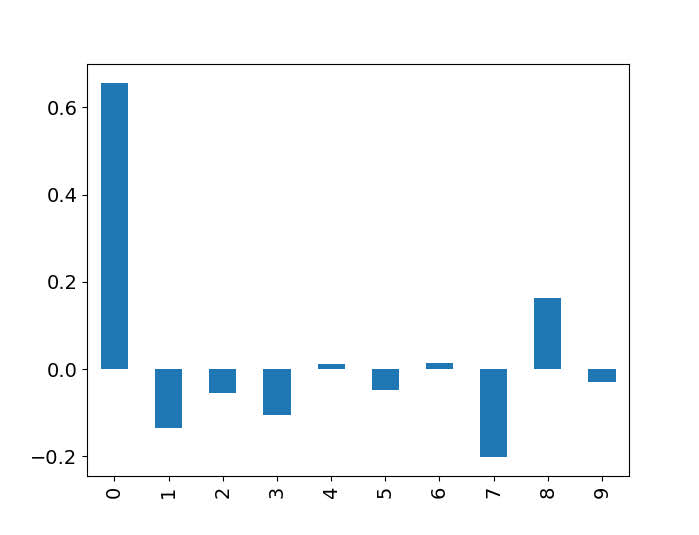

So based on this, I subsequent only look at 1 lag in subsequent models. (Prior week impacts current week, since we are analyzing weekly data.)

So you need to be careful here – typically we want to avoid doing regression analysis of integrated time series, as that can lead to spurious correlations. But in the case a series is co-integrated, it is ok to conduct analysis on the levels. So here we do the analysis of the levels for each of the securities to assess our hypothesis. (Including temporal trends results in different coefficients, but similar overall inferences.)

mod = VAR(sdat)
res = mod.fit(1) #trend='ctt'
res.summary()

So we can see here that contrary to the graphs, Ethereum has a negative relationship with BitCoin – when Ethereum goes up a dollar, the following week BitCoin goes down $1.7. For BitCoin the relationships with S&P is negative (but weaker), and Gold it is positive.

# Ethereum causes BitCoin to go down
irf = res.irf(4)
irf.plot(orth=False,impulse='Eth',response='BitCoin')

For Ethereum the converse is not true though – BitCoin + increases Ethereum (although given that BitCoin is currently 10x the value of Eth the magnitude is smaller).

# Ethereum causes BitCoin to go down
irf = res.irf(4)
irf.plot(orth=False,impulse='Eth',response='BitCoin')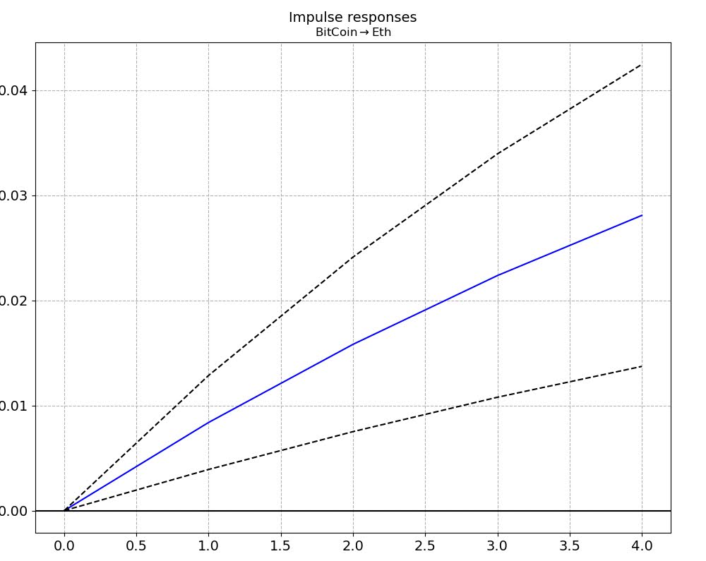

There are more formal tests to look at Granger causality and cointegration with error correction models, but looking at the VAR of the levels I think is the easiest to Grok here.

Do not take this as investment advice, looking at the volatility of these securities makes me very hesistant to invest even a small sum.

# Granger causality test
gc = res.test_causality('Eth', 'BitCoin', kind='f').summary()
print(gc)

# Cointegration test
ecm = vecm.coint_johansen(sdat[['BitCoin','Eth']], 1, 1)
print(ecm.max_eig_stat)
print(ecm.max_eig_stat_crit_vals)

ecm = vecm.VECM(sdat[['BitCoin','Eth']],deterministic='co')
est = ecm.fit()

est.plot_forecast(4,n_last_obs=10)
plt.show()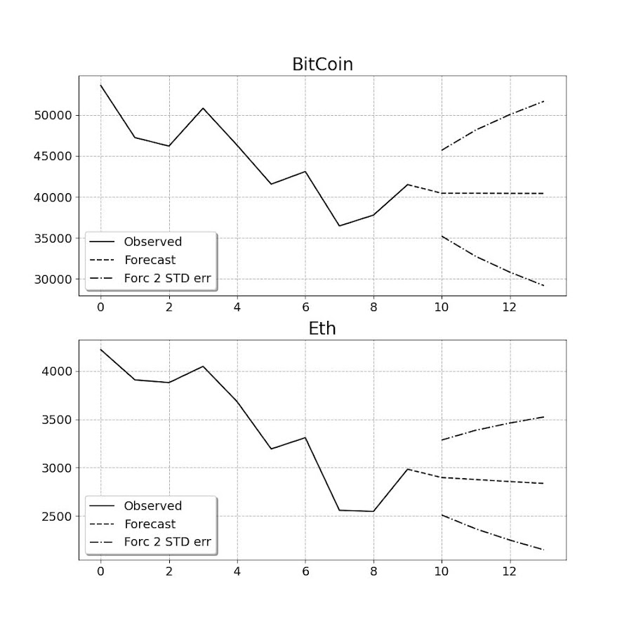

Based on this analysis it might make sense to include BitCoin as a portfolio diversification relative to traditional stocks – if willing to assume quite a bit of risk. If you are a gambler it may make sense to do some type of pairs trading strategy between Eth/Bitcoin on a short term basis. (If I had some real magic low risk money making strategy I would not put it in a blog post!)

Gambling is fun (and it is fun to think damn if I invested in Eth in 2019 I would be up 10x) – but I don’t think I am going onto the crypto roller-coaster at the moment.