

Jupyter Notebook Viewer
source link: https://nbviewer.jupyter.org/github/MokoSan/FSharpAdvent_2020/blob/main/BayesianInferenceInF%23.ipynb
Go to the source link to view the article. You can view the picture content, updated content and better typesetting reading experience. If the link is broken, please click the button below to view the snapshot at that time.
Bayesian Inference in FSharp
Introduction
For my F# Advent submission this year, I decided to implement an extremely simple Bayesian Statistical Framework to be used for inference. The purpose of statistical inference is to infer characteristics of a population via samples. The "Bayesian" prefix refers to making use of the Bayes Theorem to conduct inferential statistics.
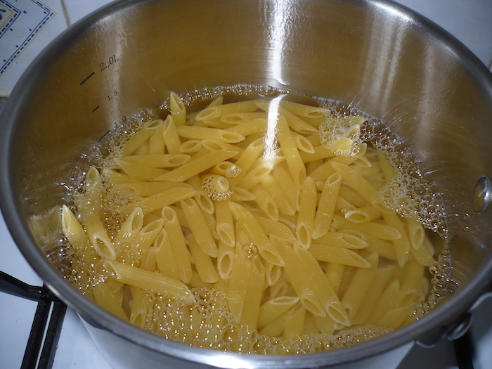
I like to think of Statistical Inference via a pasta cooking analogy: hypothetically, assume you lose the cooking instructions of dried pasta you are trying to cook. You start boiling the water and don't know when the pasta is al-dente. One way to check is to careful remove a piece or two and test if it is cooked to your liking. Through this process, you'll know right away if the pasta needs to cook more or is ready to be sauce'd up. Similarly, inference deals with trying to figure out characteristics (is the pasta ready?) of a population (all the pasta) via samples (a single or few pieces of the pasta of your choice).
F#, as a language, didn't fail to deliver an awesome development experience! Admittedly, I hadn't used F# much in the past couple of months because of my deep dives into R and Python. However, within little to no-time a combination of muscle memory and ease of usage bumped up my productivity. The particular aspects of the language that made it easy to develop a Bayesian Statistical Framework are Pattern Matching and Immutable Functional Data Structures such as Records and Discriminated Unions that make expressing the domain succinctly and lucidly not only for the developer but also the reader.
Motivation
I recently received a Masters in Data Science but discovered that none of my courses dove deep into Bayesian Statistics. Therefore, motivated by a penchant desire to fully understand the differences between frequentist approaches and Bayesian ones to eventually gain an understanding of Bayesian Neural Networks. I, consequently, set out to dive deep into the world of Bayesian Statistics.
While reading "A First Course in Bayesian Statistical Methods" by Peter Hoff (highly recommend this book to those with a strong mathematical background) and this playlist by Ben Lambert, I discovered pymc3, a Probabilistic Programming library in Python. Pymc3, in my opinion, has some great abstractions that I wanted to implement myself in a functional-first setting.
The best way to learn a new statistical algorithm is my implementing it and the best way to learn something well is to teach it to others; this submission is a result of that ideology.
Bayes Theorem
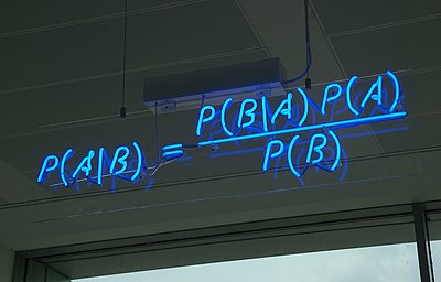
The crux of Bayesian Inference lies in making use of the Bayes Theorem to get the Posterior:
From an inferential perspective, here are the interpretations of the terms of theorem:
Term Mathematical Representation Definition Variable to Infer θθ The variable we are trying to infer details about from a population i.e. trying to figure out if that variable is characteristic of the population. Observations yy Observations obtained to validate our hypothesis that θθ is characteristic of the true population. Prior p(θ)p(θ) The likelihood of the hypothesis that θθ represents the true population before obtaining any observations Likelihood p(y∣θ)p(y∣θ) Also known as the Sampling Model, is the likelihood that yy would be the outcome of our experiment if we knew θθ was representative of the true population. Evidence p(y)p(y) Likelihood of observing the data we have collected in all circumstances regardless of our hypothesis. This quantity can also be interpretted as the normalizing constant that causes our posterior probability to be a real number between 0.0 and 1.0. It's important to note that this quantity, out of the box, doesn't depend on the variable we are trying to infer. Posterior p(θ∣y)p(θ∣y) Likelihood of our hypothesis that θθ is characteristic of the true population after observing the data or in light of new information.In my opinion, Bayes Theorem resonates with the Scientific Method as we are effectively trying to quantify the validity of a hypothesis in light of new information i.e. compute the posterior distribution. As an important observational aside, the type of the output of Bayes Theorem i.e. the type of is a probability distribution rather than a point-estimate, which has some consequences in practice.
Bayesian Inference in Practice
In practice, the denominator or the Evidence i.e. the normalization constant of the Bayes theorem is a pain to calculate. For example, for continuous variables, Bayes theorem has the following form via an application of the Law of Total Probability:
That integral in the denominator is UGLY and sometimes computational infeasible and so, approximation techniques must be used to get to generate the posterior distribution: enter Markov-Chain Monte Carlo (MCMC) methods taking advantage of the fact that the denominator is a normalization constant i.e. the posterior isn't proportional to the evidence but is proportional to the product of the prior and likelihood:
Markov-Chain Monte-Carlo (MCMC) Algorithms
MCMC algorithms help avoid the issue of the ugly sometimes infeasible denominator of Bayes Theorem by giving us approximations of the posterior distribution. For the sake of clarity to give a definition for these algorithms, let's break up the conjugated terms:
Monte-Carlo
This term refers to fact that we make use of random numbers via a random number generator to approximate the posterior distribution to some reasonable degree of precision. The premise for the use of the Monte-Carlo method is that of the Law of Large Numbers, which states that the average of the results of an experiment of a large number of iterations or trials tends to get closer to the expected value.
The use case here is the large number of iterations guided by random number generators to cleverly approximate the posterior distribution will eventually resemble the posterior distribution.
Markov-Chain
"The future only depends on the present, not the past" - Peter Hoff (knicked this from Peter Hoff's AWESOME book mentioned before) encapsulates the idea behind Markov-Chains. Markov-Chains are a sequence of events whose probability is only a function of the previous event. To a computer scientist, a Markov-Chain can be thought of as a linked list (Thanks Steve!) of approximations whose values via Monte-Carlo methods typify the posterior.
Metropolis Hastings Algorithm
The Metropolis Hastings Algorithm is one choice of a MCMC Algorithm that can be used to approximate the posterior distribution. This algorithm, for each chain in the Markov-Chains, decides at each step or iteration if a random move in parameter space to approximate the posterior is worth keeping or rejecting based on a criteria that'll describe later. The specific flavor of Metropolis Hastings I make use of is the Symmetric Metropolis Hastings algorithm and I'll elucidate on its implementation in a section below.
Goals
The goals of this submission are to develop the following:
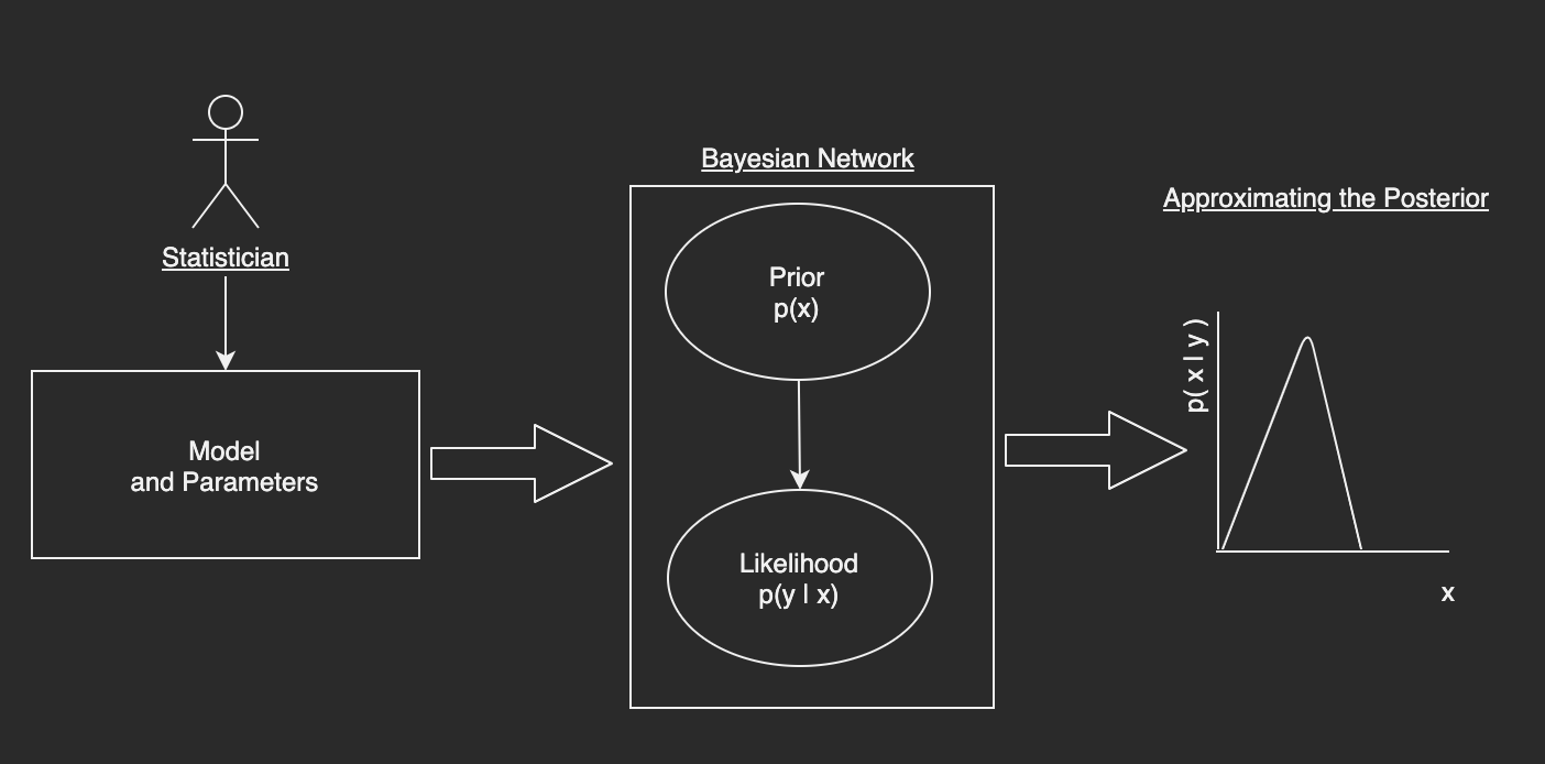
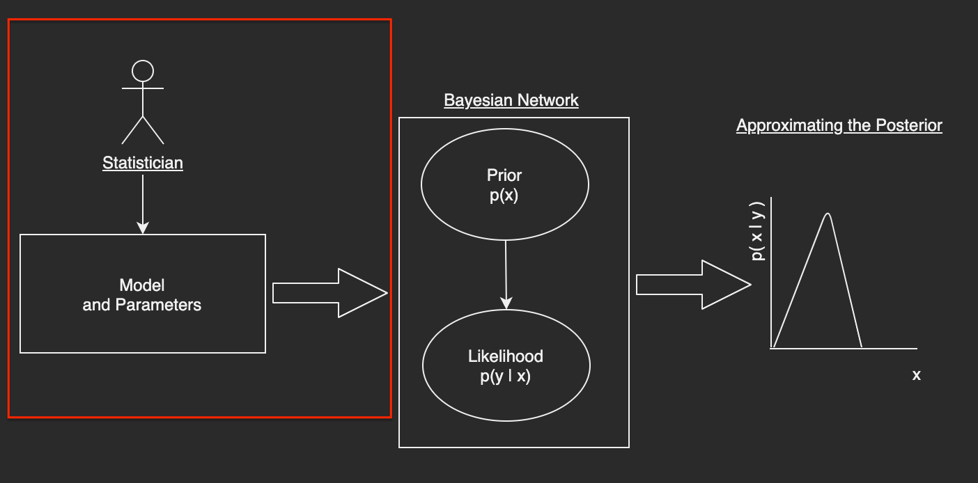
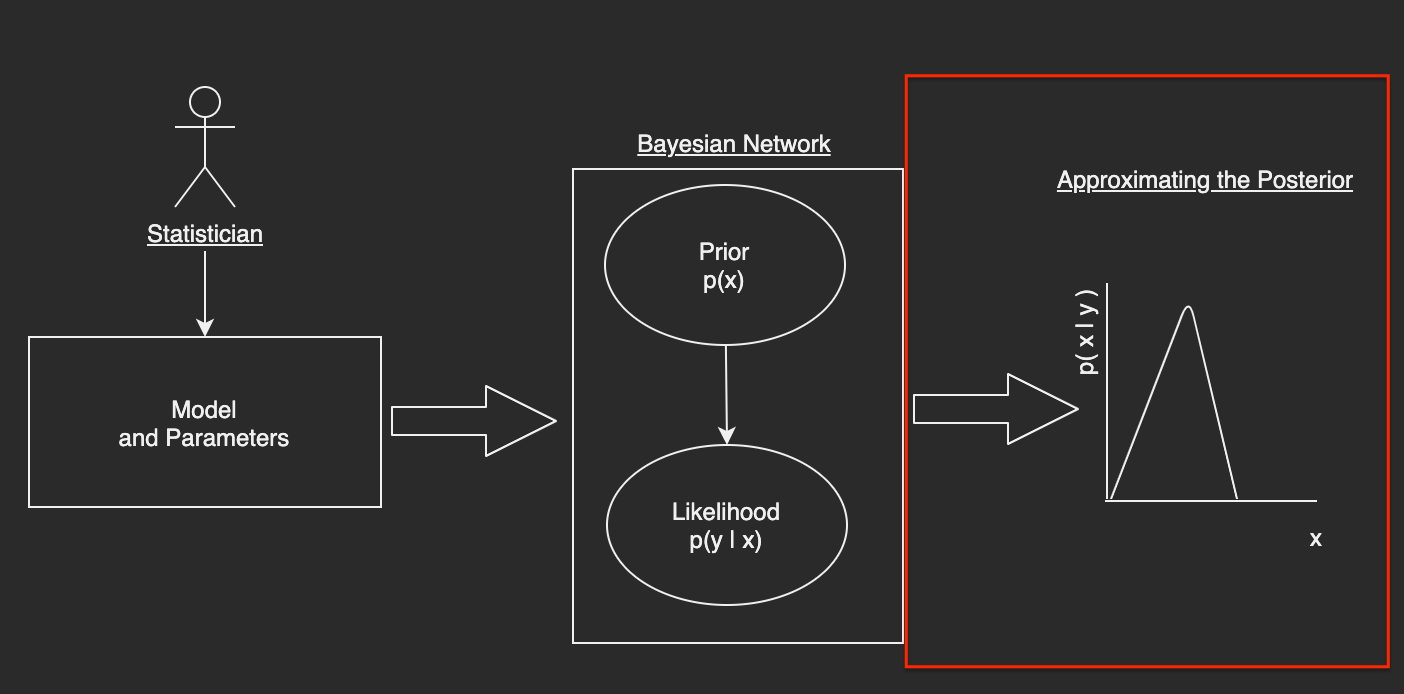
- A Bayesian Domain Specific Language (DSL) and Its Parser that a statistician with no programming experience can understand and use to specify a model and its parameters. Once our user specifies the model and the parameters, the parser associated with the Bayesian DSL converts this model into something digestable by the framework.
- A Bayesian Network from the Parsed Bayesian DSL addressing the simplest case i.e. one random variable representing the prior and one for the likelihood in the form of a Directed Acylical Graph (DAG).
- Symmeteric Metropolis-Hastings, an MCMC algorithm that makes use of the Bayesian DSL representation to approximate the posterior distribution.
Here is the proposed workflow I have developed in this submission; I will continue to add to it as time goes on but it is a start:
Getting Setup
The inferential logic will require minimal dependencies:
Dependency Use XPlot.Plotly Used for charting the histogram of the distributions. MathNet.Numerics Used for the out-of-the-box statistical distributions. Newtonsoft.Json Parsing the parameters of the Bayesian DSL.I wrote this notebook via the .net-fsharp kernel via .NET Interactive and found it great to use! This blogpost was pretty helpful to get me started.
// Dependencies
#r "nuget: XPlot.Plotly"
#r "nuget: MathNet.Numerics"
#r "nuget: Newtonsoft.Json"

// Imports
open XPlot.Plotly
open MathNet.Numerics
open Newtonsoft.Json
A Bayesian Domain Specific Language (DSL) and Its Parser
The goal of this section is to develop a Bayesian Domain Specific Language (DSL) that a statistician with no programming experience can understand and use to specify a model and its parameters.
Drawing inspiration from Stan and pymc3 tutorials such as this one, I wanted this DSL to be extremely simple, albeit, complete and therefore, the components I found that describe each random variable of the Bayesian Model are:
- The Name of the Random Variable
- Conditionals of the Random Variables i.e. what other variables are given to be true to completely specify the random variable
- The distribution associated with the random variable.
- The parameters as variables of the distribution e.g. for a Normal Distribution, the parameters will be μμ and σσ, the mean and the variance respectively.
- The observed data for the Random Variable - if the random variable has
- A map of the parameters to constants to decouple the model from the values associated with the model.
I also wanted this DSL to be a first class citizen in the eyes of a Bayesian statistician that specifies models using probability distributions.
Format
Random Variable Name [|Comma-separated Conditionals] ~ Distribution(Comma-separated Parameters without spaces) [: observed]The details enclosed in [] imply optionality.
Example
θ ~ Gamma(a,b)
Y|θ ~ Poisson(θ) : observed1
Z|Y,θ ~ Beta(θ, Y) : observed2
The Domain
The domain or the types associated with the representation of the ParsedRandomVariable representing a single line in the specified model and the ParsedBayesianModel is a list of these.
type ParsedRandomVariable =
    { Name             : string
      Conditionals     : string list
      Distribution     : string
      Parameters       : string list
      Observed         : string option }

type ParsedBayesianModel = ParsedRandomVariable list
Parsing Logic
The parsing logic for each line in the user specified model is as follows:
- Split the line by spaces.
- Extract the Name and the Conditionals from the first part of the model split on the tilde (~).
Random Variable Name | [Conditionals]. - From the second part of the model split on the tilde, get the name of the distribution and its associated parameters along with the optionally available observed variable.
F#'s awesome pattern matching was a lifesaver here not only for it's ease of use but it's automatic ability to specify the failure cases.
open System

// Format: RVName [|Conditionals] ~ Distribution(Parameters) [: observed]
// [] -> optional
// NOTE: There can't be any spaces in the distribution parameters.
let parseLineOfModel (lineInModel : string) : ParsedRandomVariable =

    // Helper fn to split the string based on a variety of type of delimiters.
    // Resultant type is a list of strings to feed in for the pattern matching.
    let splitToList (toSplit : string) (delimiters : obj) : string list =
        let split =
            match delimiters with
            | :? string        as s   -> toSplit.Split(s, StringSplitOptions.RemoveEmptyEntries)
            | :? array<string> as arr -> toSplit.Split(arr, StringSplitOptions.RemoveEmptyEntries)
            | :? array<char>   as arr -> toSplit.Split(arr, StringSplitOptions.RemoveEmptyEntries)
            | _ -> failwithf "Splitting based on delimiters failed as it is neither a string nor an array of strings: Of Type: %A - %A" (delimiters.GetType()) toSplit

        Array.toList split

    match splitToList lineInModel " " with
    | nameAndConditionals :: "~" :: distributionParametersObserved ->
        // Get the name and conditionals.
        let splitNameAndConditionals = splitToList nameAndConditionals "|"
        let name = splitNameAndConditionals.[0]
        let conditionals =
            match splitNameAndConditionals with
            | name :: conditionals ->
                if conditionals.Length > 0 then splitToList conditionals.[0] ","
                else []
            | _ -> failwithf "Pattern not found for RV Name and Conditionals - the format is: RVName|Condtionals: %A" splitNameAndConditionals

        let extractAndGetParameters (distributionNameAndParameters : string) : string * string list =
            let splitDistributionAndParameters = splitToList distributionNameAndParameters [| "("; ")" |]
            (splitDistributionAndParameters.[0], splitToList splitDistributionAndParameters.[1] ",")

        match distributionParametersObserved with

        // Case: Without Observations. Example: θ ~ Gamma(a,b)
        | distributionNameAndParameters when distributionNameAndParameters.Length = 1 ->
            let extractedDistributionAndParameters = extractAndGetParameters distributionNameAndParameters.[0]
            { Name             = name;
              Conditionals     = conditionals;
              Distribution     = (fst extractedDistributionAndParameters).ToLower();
              Observed         = None;
              Parameters       = snd extractedDistributionAndParameters; }

        // Case: With Observations. Example: Y|θ ~ Poisson(θ) : observed
        | distributionNameAndParameters :: ":" :: observed ->
            let extractedDistributionAndParameters = extractAndGetParameters distributionNameAndParameters
            { Name             = name;
              Conditionals     = conditionals;
              Distribution     = (fst extractedDistributionAndParameters).ToLower();
              Observed         = Some observed.Head; // Only 1 observed list permitted.
              Parameters       = snd extractedDistributionAndParameters; }

        // Case: Error.
        | _ -> failwithf "Pattern not found for the model while parsing the distribution, parameters and optionally, the observed variables: %A" distributionParametersObserved

    | _ -> failwithf "Pattern not found for the following line in the model - please check the syntax: %A" lineInModel

let parseModel (model : string) : ParsedBayesianModel =
    model.Split('\n')
    |> Array.map(parseLineOfModel)
    |> Array.toList

// Helper to print out the Parsed Bayesian Model
let printParsedModel (model : string) : unit =
    let parsedModel = parseModel model
    printfn "Model: %A is represented as %A" model parsedModel
Examples of Parsing a User-Specified DSL
// Print out our simple 1-Parameter Model.
let model1 = @"θ ~ Gamma(a,b)
              Y|θ ~ Poisson(θ) : observed"
printParsedModel(model1)

// This model doesn't make sense but adding to test multiple conditionals.
let model2  = @"θ ~ Beta(unit,unit)
               γ ~ Gamma(a,b)
               Y|θ,γ ~ Binomial(n,θ) : observed"
printParsedModel(model2)
Model: "θ ~ Gamma(a,b)
              Y|θ ~ Poisson(θ) : observed" is represented as [{ Name = "θ"
   Conditionals = []
   Distribution = "gamma"
   Parameters = ["a"; "b"]
   Observed = None }; { Name = "Y"
                        Conditionals = ["θ"]
                        Distribution = "poisson"
                        Parameters = ["θ"]
                        Observed = Some "observed" }]
Model: "θ ~ Beta(unit,unit)
               γ ~ Gamma(a,b)
               Y|θ,γ ~ Binomial(n,θ) : observed" is represented as [{ Name = "θ"
   Conditionals = []
   Distribution = "beta"
   Parameters = ["unit"; "unit"]
   Observed = None }; { Name = "γ"
                        Conditionals = []
                        Distribution = "gamma"
                        Parameters = ["a"; "b"]
                        Observed = None }; { Name = "Y"
                                             Conditionals = ["θ"; "γ"]
                                             Distribution = "binomial"
                                             Parameters = ["n"; "θ"]
                                             Observed = Some "observed" }]
Specifying the Parameters
The idea is to decouple the parameters separate from the model and this is done by saving the details as a JSON string. This task is made simple using the Newtonsoft.Json library.
open System
open System.Collections.Generic

open MathNet.Numerics.Distributions

open Newtonsoft.Json

type Observed = float list

type ParameterList =
    { Observed : float list; Parameters : Dictionary<string, float> }

let deserializeParameters (paramsAsString : string) : ParameterList =
    JsonConvert.DeserializeObject<ParameterList>(paramsAsString)
Examples of the Deserialization of the Parameters
// Parameter List 1
let parameters1 = "{Parameters : {μ0 : 0, σ0 : 1, μ : 5, σ : 2, λ : 4}, observed : [4.2,0.235,2.11]}"
let deserializedParameters1 = deserializeParameters parameters1
printfn "Deserialized Parameters 1: %A" (deserializedParameters1)

// Parameter List 2
let parameters2 = "{Parameters: {λ : 2}}"
let deserializedParameters2 = deserializeParameters parameters2
// Applying the Deserialized Parameters to Sample from a Distribution
let exp = Exponential deserializedParameters2.Parameters.["λ"]
printfn "Sampling from the Exponential Distribution with the λ = %A parameter: %A" exp (exp.Sample())
Deserialized Parameters 1: { Observed = [4.2; 0.235; 2.11]
  Parameters = seq [[μ0, 0]; [σ0, 1]; [μ, 5]; [σ, 2]; ...] }
Sampling from the Exponential Distribution with the λ = Exponential(λ = 2) parameter: 1.673949327
Converting the Parsed Model into a Bayesian Network

The goal is to take the parsed representations of the user-inputted model and convert them into a directed acylic graph (DAG) that represents a Bayesian Network in an effort to easily and generically compute the posterior distribution.
The first step here is to map the distribution that's specified by the user as a string to an actual function that can compute the density or mass functions used in the prior and likelihood calculations. Subsequent to the distribution mapping, creating the notion of a Bayesian Node and the associated Bayesian Network will lead us to having a concrete form of the specified model. In this flavor of implementation, I will be simplifying the logic to only consider a two node network with one node representing the prior and the other, the likelihood. In a future post, I'll be generalizing this algorithm further.
Distribution Mapping
The distribution mapping step involves developing:
- Type-specified domain for the distribution.
- Parsing logic that takes the name of the distribution and applies the ParsedRandomVariable based parameters to it.
- A helper function based on the type of distribution to get the probability density function based on an input.
NOTE: The list of distributions is incomplete, however, the idea should be similar to add newer ones.
open MathNet.Numerics.Distributions

type DistributionType =
    | Continuous
    | Discrete

type Parameter     = float
type DiscreteInput = int
type Input         = float

type DensityType =
    | OneParameter         of (Parameter * Input -> float)
    | OneParameterDiscrete of (Parameter * DiscreteInput -> float)
    | TwoParameter         of (Parameter * Parameter * Input -> float)

type DistributionInfo = { RVName             : string
                          DistributionType   : DistributionType
                          DistributionName   : string
                          Parameters         : float list
                          Density            : DensityType } with

    static member Create (item : ParsedRandomVariable)
                         (parameterList : ParameterList) : DistributionInfo =
    // I know this is ugly but this functionality assumes the user enters the
    // parameters in the order that's expected by the MathNet Numerics Library.
    // Grab the parameters associated with this Random Variable.
    let rvParameters =
        item.Parameters
        |> List.filter(parameterList.Parameters.ContainsKey)
        |> List.map(fun item -> parameterList.Parameters.[item])

    // Extract Distribution Associated with the Parsed Random Variable.
    match item.Distribution with

    // 1 Parameter Distributions
    | "exponential" ->
        { RVName           = item.Name
          DistributionName = item.Distribution
          Parameters       = rvParameters
          DistributionType = DistributionType.Continuous
          Density          = OneParameter Exponential.PDF }
    | "poisson" ->
        { RVName           = item.Name
          DistributionName = item.Distribution
          Parameters       = rvParameters
          DistributionType = DistributionType.Discrete
          Density          = OneParameterDiscrete Poisson.PMF }
    // 2 Parameter Distributions
    | "normal" ->
        { RVName           = item.Name
          DistributionName = item.Distribution
          Parameters       = rvParameters
          DistributionType = DistributionType.Continuous
          Density          = TwoParameter Normal.PDF }
    | "gamma" ->
        { RVName           = item.Name
          DistributionName = item.Distribution
          Parameters       = rvParameters
          DistributionType = DistributionType.Continuous
          Density          = TwoParameter Gamma.PDF }
    | "beta" ->
        { RVName           = item.Name
          DistributionName = item.Distribution
          Parameters       = rvParameters
          DistributionType = DistributionType.Continuous
          Density          = TwoParameter Beta.PDF }
    | "continuousuniform" ->
        { RVName           = item.Name
          DistributionName = item.Distribution
          Parameters       = rvParameters
          DistributionType = DistributionType.Continuous
          Density          = TwoParameter ContinuousUniform.PDF }
    // Failure Case
    | _ -> failwithf "Distribution not registered: %A" item.Distribution

    member this.ComputeOneParameterPDF (parameter : float) (input : float) : float =
        match this.Density with
        | OneParameter pdf -> pdf(parameter,input)
        | _ -> failwithf "Incorrect usage of function with a non One Parameter Density Type. Density given: %A" this.Density
    member this.ComputeOneParameterDiscretePMF (parameter : float) (input : int) : float =
        match this.Density with
        | OneParameterDiscrete pmf -> pmf(parameter,input)
        | _ -> failwithf "Incorrect usage of function with a non One Parameter Discrete Density Type. Density given: %A" this.Density
    member this.ComputeTwoParameterPDF (parameter1 : float) (parameter2 : float) (input : float) : float =
        match this.Density with
        | TwoParameter pdf -> pdf(parameter1, parameter2, input)
        | _ -> failwithf "Incorrect usage of function with a non Two Parameter Density Type. Density given: %A" this.Density
Helper Methods to get the Distributions from the User Specified DSL
let getDistributionInfoForModel(model : string) (parameterList : string) : DistributionInfo list =
    let parsedModel   = parseModel model
    let parameterList = deserializeParameters parameterList
    parsedModel
    |> List.map(fun x -> DistributionInfo.Create x parameterList)

let getDensityOrProbabilityForModel (model : string)
                                    (parameterList : string)
                                    (data : float seq) : IDictionary<string, float seq> =
    getDistributionInfoForModel model parameterList
    |> List.map(fun (e : DistributionInfo) ->
        match e.Density with
        | OneParameter p ->
            let param   = List.exactlyOne e.Parameters
            let results = data |> Seq.map(fun d -> e.ComputeOneParameterPDF param d)
            e.RVName, results
        | OneParameterDiscrete p ->
            let param   = List.exactlyOne e.Parameters
            let results = data |> Seq.map(fun d -> e.ComputeOneParameterDiscretePMF param (int d))
            e.RVName, results
        | TwoParameter p ->
            let p2 : float list = e.Parameters |> List.take 2
            let results = data |> Seq.map(fun d -> e.ComputeTwoParameterPDF p2.[0] p2.[1] d)
            e.RVName, results)
    |> dict
Testing the Distribution Mapping Logic on Random Samples via a Simple Model
// Exponential.
let exponentialModel     = "x ~ Exponential(lambda)"
let exponentialParamList = "{Parameters: {lambda : 2, a : 2., b : 2.3}, Observed : []}"
let exponentialDummyData = ContinuousUniform.Samples(0., 200.) |> Seq.take 2000
let exponentialPdfs      = getDensityOrProbabilityForModel exponentialModel exponentialParamList exponentialDummyData
printfn "Exponential: %A" (exponentialPdfs.Values)

// Normal.
let normalModel     = "x ~ Normal(mu,sigma)"
let normalParamList = "{Parameters: {mu: 0., sigma : 1.}, Observed : []}"
let normalDummyData = Normal.Samples(0.0, 1.0) |> Seq.take 2000
let normalPdfs      = getDensityOrProbabilityForModel normalModel normalParamList normalDummyData
printfn "Normal: %A" (normalPdfs.Values)

// Poisson.
let poissonModel     = "x ~ Poisson(theta)"
let poissonParamList = "{Parameters: {theta: 44}, Observed : []}"
let poissonDummyData = ContinuousUniform.Samples(0., 5.) |> Seq.take 2000
let poissonPdfs      = getDensityOrProbabilityForModel poissonModel poissonParamList poissonDummyData
printfn "Poisson: %A" (poissonPdfs.Values)
Exponential: seq
  [seq [5.021224175e-54; 6.790246353e-50; 2.044679134e-68; 2.02863983e-172; ...]]
Normal: seq [seq [0.3813916696; 0.1382035578; 0.1331370548; 0.2884060033; ...]]
Poisson: seq
  [seq [1.104713281e-15; 1.21518461e-14; 7.532136009e-17; 1.21518461e-14; ...]]
Bayesian Node
The next step is to specify the Bayesian Node, the abstraction that should encapsulate all the information for successfully computing probabilities. There can be two types of Nodes:
- With Observed Variables for cases such as the Likelihood where we have data from a sampling model.
- Non-Observed Variables for cases such as the Prior where all we have is a guess as to what the distribution of the parameter we want to infer is.
type BayesianNodeTypeInfo =
    | Observed of float list
    | NonObserved

type BayesianNode =
    { Name                 : string
      NodeType             : BayesianNodeTypeInfo
      DistributionInfo     : DistributionInfo
      ParsedRandomVariable : ParsedRandomVariable } with

    static member Create(parsedRandomVariable : ParsedRandomVariable)
                        (parameterList : ParameterList) =

        let nodeType : BayesianNodeTypeInfo =
            match parsedRandomVariable.Observed with
            | Some _ -> BayesianNodeTypeInfo.Observed parameterList.Observed
            | None   -> BayesianNodeTypeInfo.NonObserved
        { Name                 = parsedRandomVariable.Name;
          NodeType             = nodeType;
          DistributionInfo     = DistributionInfo.Create parsedRandomVariable parameterList;
          ParsedRandomVariable = parsedRandomVariable; }

    member this.GetDependents (parsedBayesianModel : ParsedBayesianModel) : ParsedRandomVariable list =
        parsedBayesianModel
        |> List.filter(fun x -> x.Conditionals |> List.contains(this.Name))
An Example of Creating a Node From a Line in the Model
let lineOfModel = @"x ~ Exponential(lambda) : observed"
let paramList   = "{Parameters: {lambda : 2, a : 2., b : 2.3 }, observed : [1,2,3,55]}"
BayesianNode.Create (parseLineOfModel lineOfModel) (deserializeParameters paramList)
Simple Bayesian Network
A General Bayesian Network is a Directed Acyclic Graph consisting of Bayesian Nodes and the relationship amongst them. A Simple Bayesian Network is a type of Bayesian Network with two Bayesian Nodes namely, the Prior and Likelihood nodes or in other words, the model that the user can specify is constrained to two random variables; this is done for the sake of simplicity.
The Simple Bayesian Network also consists of functions that can be used to compute the numerator of Bayes Theorem i.e. Posterior=Prior×LikelihoodPosterior=Prior×Likelihood
The Prior is computed using the PDF or PMF based on the parameters associated with the Prior Bayesian Node. For example, a Normal Prior Node will have the formula of Normal.PDF(mean, stddev, input).
The Likelihood, on the other hand, involves the result from the Prior and the observed list. The assumptions in the computation of the Likelihood is that the observations are conditionally independent given our prior and the exchangability of the observations where the order of the observations don't matter i.e. the order or labels of the observations don't change the outcome.
In other words, we will be computing the PDF based on the prior, parameters of the likelihood node and the observed variables. For example, if we were to be inferring the mean of the Normal distribution, our likelihood will be computed by the following pseudo-code: product(Normal.PDF(prior, stddevOfLikelihood, observation))
// Only to be used for a model with 2 nodes
// i.e. one for the prior and one for the likelihood.
type SimpleBayesianNetworkModel =
  { Name       : string
    Nodes      : IDictionary<string, BayesianNode>
    Prior      : BayesianNode
    Likelihood : BayesianNode } with

    member this.GetPriorProbability (input : float) : float =
      let distributionInfo = this.Prior.DistributionInfo
      match distributionInfo.Density with
      | OneParameter p ->
          let param = List.exactlyOne distributionInfo.Parameters
          distributionInfo.ComputeOneParameterPDF param input
      | OneParameterDiscrete p ->
          let param   = List.exactlyOne distributionInfo.Parameters
          distributionInfo.ComputeOneParameterDiscretePMF param (int input)
      | TwoParameter p ->
          let p2 : float list = distributionInfo.Parameters |> List.take 2
          distributionInfo.ComputeTwoParameterPDF p2.[0] p2.[1] input

    member this.GetLikelihoodProbability (prior : float) : float =
        let distributionInfo = this.Likelihood.DistributionInfo
        let observed         = match this.Likelihood.NodeType with
                               | Observed l -> l
                               | _ -> failwithf "Incorrectly constructed Simple Network Model. %A" this
        let density =
          match distributionInfo.Density with
          | OneParameter p ->
              observed |> List.map(fun d -> distributionInfo.ComputeOneParameterPDF prior d)
          | OneParameterDiscrete p ->
              observed |> List.map(fun d -> distributionInfo.ComputeOneParameterDiscretePMF prior (int (Math.Ceiling d)))
          | TwoParameter p ->
              let p : float = distributionInfo.Parameters |> List.exactlyOne
              observed |> List.map(fun d -> distributionInfo.ComputeTwoParameterPDF prior p d)
        density
        |> List.fold (*) 1.0

    member this.GetPosteriorWithoutScalingFactor (input: float) : float =
      let priorPdf      = this.GetPriorProbability input
      let likelihoodPdf = this.GetLikelihoodProbability priorPdf
      priorPdf * likelihoodPdf

    static member Construct (name : string)
                            (model : ParsedBayesianModel)
                            (parameterList : ParameterList) : SimpleBayesianNetworkModel =

        // Construct all the modes of the model.
        let allNodes : (string * BayesianNode) list =
            model
            |> List.map(fun m -> m.Name, BayesianNode.Create m parameterList)

        let prior : BayesianNode =
            allNodes
            |> List.filter(fun (_,m) -> m.NodeType = BayesianNodeTypeInfo.NonObserved)
            |> List.map(fun (_,m) -> m)
            |> List.exactlyOne

        let likelihood : BayesianNode =
            allNodes
            |> List.filter(fun (_,m) -> m.NodeType <> BayesianNodeTypeInfo.NonObserved)
            |> List.map(fun (_,m) -> m)
            |> List.exactlyOne

        { Name       = name;
          Nodes      = dict allNodes;
          Prior      = prior;
          Likelihood = likelihood; }
Example of Creating a Simple Bayesian Network
let model = @"x ~ Normal(μ,τ)
              y|x ~ Normal(x,σ) : observed"
let parsedModel = parseModel model
let paramList = "{Parameters: {μ : 5, τ : 3.1622, σ : 1}, observed : [9.37,10.18,9.16,11.60,10.33]}"
let normalModel =
    SimpleBayesianNetworkModel.Construct "Normal-Normal" parsedModel (deserializeParameters paramList)
normalModel
Debugging the Prior and Likelihood
A quick sanity check to see if the numbers match up if we were to compute the Prior and Likelihood "by hand".
let model = @"x ~ Normal(μ,τ)
              y|x ~ Normal(x,σ) : observed"
let parsedModel = parseModel model
let paramList = "{Parameters: {μ : 5, τ : 3.1622, σ : 1}, observed : [9.37,10.18,9.16,11.60,10.33]}"
let normalModel =
    SimpleBayesianNetworkModel.Construct "Normal-Normal" parsedModel (deserializeParameters paramList)

// Prior Check
let priorFromModel = normalModel.GetPriorProbability 0.0
let computedPrior  = Normal.PDF(5., 3.1622, 0.0)
printfn "Normal Model Prior: %A | Prior from formula: %A" priorFromModel computedPrior

// Likelihood Check
let likelihoodFromModel = normalModel.GetLikelihoodProbability 0.0
let observed : float list =
    match normalModel.Likelihood.NodeType with
    | Observed x -> x
    | _ -> failwithf "Incorrectly constructed Likelihood"

let likelihoodListFromFormula : float list =
    observed |> List.map(fun (o:float) -> Normal.PDF(computedPrior, 1., o))
let likelihoodFromFormula = likelihoodListFromFormula |> List.fold (*) 1.

printfn "Normal Model Likelihood: %A | Likelihood from formula: %A"
    (normalModel.GetLikelihoodProbability 0.03614314702)
    (likelihoodFromFormula)
Normal Model Prior: 0.03614314702 | Prior from formula: 0.03614314702
Normal Model Likelihood: 4.158402902e-114 | Likelihood from formula: 4.158402901e-114
Applying the Symmetric Metropolis Hastings Algorithm to Approximate the Posterior Distribution
Now that we have some digestible representation of the Simple Bayesian Network, our next step is to make use of an MCMC algorithm to approximate the posterior. The steps here as follows:
- Define a well-specified MCMC domain to run the algorithmss.
- Implement a type of MCMC algorithm called the Symmetric Metropolis Hasting Algorithm.
- Apply the algorithm to a Simple Bayesian Network.
The Symmetric Metropolis Hastings Algorithm
I would consider the Symmetric Metropolis Hastings Algorithm to be a simple MCMC algorithm that's based on some smart applications of the Bayes Theorem and therefore, I chose it to be the "toy" approximation algorithm used here. There are better algorithms out there such as Hamiltonian Monte-Carlo or the No U-Turn Sampler that I plan to prospectively explore.
The Algorithm
- Produce a proposal based on the proposal distribution and the current value.
- Compute the Posterior with the proposal and the current value.
- Compute the Acceptance Ratio.
- Accept or Reject the proposal. If accepted, the current value will be the proposed value else, grab another proposal using the proposal distribution.
- Repeat until iterative convergence for all chains requested.
The main ideas associated with the steps or single iterations of this algorithm are:
1. Proposing New Values To Approximate the Parameter Space
Using a proposal distribution, we come up with newer values of the parameter to explore and find regions that are more likely to be outputted by the posterior distribution. Examples of the proposal distributions are:
Uniform(current - δ, current + δ)Normal(current, δ^2)
where δ is a hyperparameter that's a proxy of the size of the jumps.
2. Computing the Acceptance Ratio
Taking advantage of the notion below and considering different parameters, say θθ and θ∗θ∗, we come up with a new quantity called the Acceptance Ratio, rr.
p(θ∣y)∝p(y∣θ)p(θ)p(θ∣y)∝p(y∣θ)p(θ)
Where r=p(θ∣y)p(θ∗∣y)=p(y∣θ)p(θ)p(y∣θ∗)p(θ∗)r=p(θ∣y)p(θ∗∣y)=p(y∣θ)p(θ)p(y∣θ∗)p(θ∗)
By examining this ratio, it can be made evident that if the numerator is greater than the denominator, we have an acceptance ratio > 1; this implies that the posterior without the normalization constant with θθ is higher than that with θ∗θ∗ or is a data-point more likely (or with less uncertainity) to be obtained from the posterior.
3. Accepting or Rejecting The Proposal Based on the Acceptance Ratio
The Symmetric Metropolis Hastings algorithm is a type of Metropolis Hastings algorithm where the proposal distribution between the current the proposed, new value is symmetric i.e. the probability to obtain the proposal given the current value is the same as the probability to obtain the current value given the proposal.
With this idea in mind, once we have computed the acceptance ratio, we want to check to see how likely it'll typify the posterior distribution. This can be done by taking a random drawing from a uniform distribution where the lower and upper values are 0 and 1 respectively. This idea can be elucidated on by the fact that if the proposal based posterior better approximates the real-posterior better than a random drawing from a 0-1 uniform distribution, in the long run, it'll eventually be close-enough to the real-posterior.
As mentioned before, if the proposal was accepted, we use that as the next current value to generate another proposal or else try to get another proposal in the subsequent iteration.
Weaknesses of this Algorithm
The simplicity of this model comes with costs, specifically, the dependence on the hyperparameters that have to be tuned and autocorrelation of values or if the proposed distribution is extremely close to the current value, it'll take longer to explore the entire parameter space as the jumps will be smaller. As an example of the weaknesses, I needed to experiment with a bunch of hyperparameters before I got to some semblance of the posterior distribution I was expecting in addition to increases the number of iterations.
Defining the MCMC Domain
I liked the idea of using a simple Request -> Result model from the Client-Server model to encapulate the approximation. Additionally, I drew inspiration from reading pymc3's code to come up with the following domain.
In general, I want any of the prospective MCMC algorithms to have the ability to:
- Output multiple chains that approximate the posterior.
- Have the ability to specify multiple types of "steps" or mechanisms to induce jumps in parameter space for appropriately approximating the posterior distribution.
- Outputting statistics as to how the algorithm did.
- Specifying a converge criteria after which the MCMC algorithm stops the approximation.
- An ability to pass in a proposal distribution on the basis of which jumps in the parameter space are induced.
Terminology
The Acceptance Rate is a result of an MCMC chain the proportion of the number of accepted proposals to the total number of non-burn in proposals. This metric is a proxy of how the steps are approximating the posterior.
The BurnInIterationsPct is the percent of posterior approximates to ignore; these are taken from the beginning of the chains and are representative of the first few jumps before the algorithm is at a point where it's better at approximating the posterior.
type ConvergenceCriteria =
    | IterativeConvergence of int // Number of Iterations

type ProposalDistribution =
    | Normal of float  // Normal( current, delta )
    | ContinuousUniform of float // ContinuousUniform( current - delta, current + delta )
    | PositiveContinuousUniform of float // ( x ~ Uniform( current - delta, current + delta ) if x <= 0 then 0.1 else x )

type MCMCInferenceStep =
    | SymmetricMetropolisHastings of ProposalDistribution * float

type MCMCChain =
    { Id             : int
      AcceptanceRate : float // # of Acceptances / Total # of Chain Items
      StepValues     : float seq }

type MCMCRequest =
    { StepFunction         : MCMCInferenceStep
      ConvergenceCriteria  : ConvergenceCriteria
      BurnInIterationsPct  : float
      Chains               : int
      PrintDebug           : bool }

type MCMCResult =
    { Chains         : MCMCChain seq
      MCMCRequest    : MCMCRequest }
open System
open MathNet.Numerics.Distributions
open XPlot.Plotly

type AcceptanceRejection =
    | Acceptance of float // Acceptance of the Proposal
    | Rejection  of float // Rejection of the Proposal

let doSymmetricMetropolisHastings (request : MCMCRequest)
                                  (iterations : int)
                                  (proposalDistribution : ProposalDistribution)
                                  (initialValue : float)
                                  (simpleBayesianModel : SimpleBayesianNetworkModel) : MCMCResult =

    let getChain (id : int) (request : MCMCRequest)
                 (iterations : int) (simpleBayesianModel : SimpleBayesianNetworkModel) : MCMCChain =

        let burnin         = int (Math.Ceiling(request.BurnInIterationsPct / 100. * float iterations))
        let zeroOneUniform = ContinuousUniform()

        let mutable current = simpleBayesianModel.GetPosteriorWithoutScalingFactor initialValue

        let matchedProposalDistribution (input : float) :  float =
            match proposalDistribution with
            | Normal delta            -> Normal(input, delta).Sample()
            | ContinuousUniform delta -> ContinuousUniform(input - delta, input + delta).Sample()
            | PositiveContinuousUniform delta ->
                let u = ContinuousUniform(input - delta, input + delta).Sample()
                if u <= 0. then input + 0.1 else u

        let step (iteration : int) : AcceptanceRejection =
            let proposed           = matchedProposalDistribution current
            let currentProbability = simpleBayesianModel.GetPosteriorWithoutScalingFactor current
            let proposedProbabilty = simpleBayesianModel.GetPosteriorWithoutScalingFactor proposed
            let acceptanceRatio    = Math.Min(currentProbability / proposedProbabilty, 1.)
            let uniformDraw        = zeroOneUniform.Sample()

            if request.PrintDebug then
                printfn "Chain: %A Iteration: %A - Current Probability: %A | Proposed Probability: %A | AcceptanceRatio: %A | Uniform Draw: %A | Current: %A | Proposed: %A"
                    id iteration currentProbability proposedProbabilty acceptanceRatio uniformDraw current proposed

            if uniformDraw < acceptanceRatio then (current <- proposed; Acceptance proposed)
            else Rejection current

        let stepResults : AcceptanceRejection seq =
            seq {1..iterations}
            |> Seq.map step
            |> Seq.skip burnin

        let getAcceptanceRateAndStepValues : float * float seq =

            // Compute the Acceptance Rate.
            let acceptanceRate : float =
                let totalBurninWithoutBurnin : float = float (Seq.length stepResults)
                let totalNumberOfAcceptances : float =
                    stepResults
                    |> Seq.filter(fun x ->
                        match x with
                        | Acceptance x -> true
                        | _ -> false)
                    |> Seq.length
                    |> float
                totalNumberOfAcceptances / totalBurninWithoutBurnin

            // Grab the Step Values that'll approximate the posterior.
            let stepValues =
                stepResults |> Seq.map(fun s ->
                    match s with
                    | Acceptance v -> v
                    | Rejection v -> v)

            acceptanceRate, stepValues

        let acceptanceRate, stepValues = getAcceptanceRateAndStepValues

        { Id             = id
          AcceptanceRate = acceptanceRate
          StepValues     = stepValues}

    let chains : MCMCChain seq =
        seq {1..request.Chains}
        |> Seq.map(fun id ->  getChain id request iterations simpleBayesianModel)

    { Chains      = chains
      MCMCRequest =  request }
Running the Algorithm
This method takes in a generic MCMC Request and a model and returns an MCMC Result consisting of the chain of results that have the posterior sequence as well as the acceptance rate.
let runMCMC (request : MCMCRequest)
            (model : SimpleBayesianNetworkModel) : MCMCResult =
    match request.StepFunction with
    | SymmetricMetropolisHastings (proposalDistribution,initialValue) ->
        match request.ConvergenceCriteria with
        | IterativeConvergence iterations ->
            doSymmetricMetropolisHastings request iterations proposalDistribution initialValue model
        | _ -> failwith "You need to pass in the number of iterations for the Metropolis-Hastings algorithm"
    | _ -> failwithf "Step Function Not Registered: %A" request.StepFunction
Tieing it All Together
Let's now go from a user inputted model to the results of the Symmetric Metropolis Hastings algorithm to approximate the posterior for two cases. We'll plot the results of the first chain to highlight if the algorithm did the right thing.
Exponential Prior and Exponential Likelihood
let model = @"x ~ Exponential(a)
              y|x ~ Exponential(x) : observed"
let parsedModel = parseModel model
let paramList = "{Parameters: {a : 2., b : 2.}, observed : [1,2,3,4,4,2,5,6,7,3,2,3,4,5,6,1,2,3,4,4,4,4]}"
let simpleModel = SimpleBayesianNetworkModel.Construct "Exponential Model" parsedModel (deserializeParameters paramList)

let request : MCMCRequest =
    { StepFunction        = SymmetricMetropolisHastings (ProposalDistribution.PositiveContinuousUniform 0.002, 0.001)
      ConvergenceCriteria = IterativeConvergence 10000
      BurnInIterationsPct = 0.2
      PrintDebug          = false
      Chains              = 4 }

let mcmc       = runMCMC request simpleModel
let firstChain = Seq.head mcmc.Chains

Histogram(x = firstChain.StepValues)
|> Chart.Plot
|> Chart.WithTitle "Exponential Prior and Likelihood"
As the online notebook renderer isn't displaying the chart, I took a screenshot of it.
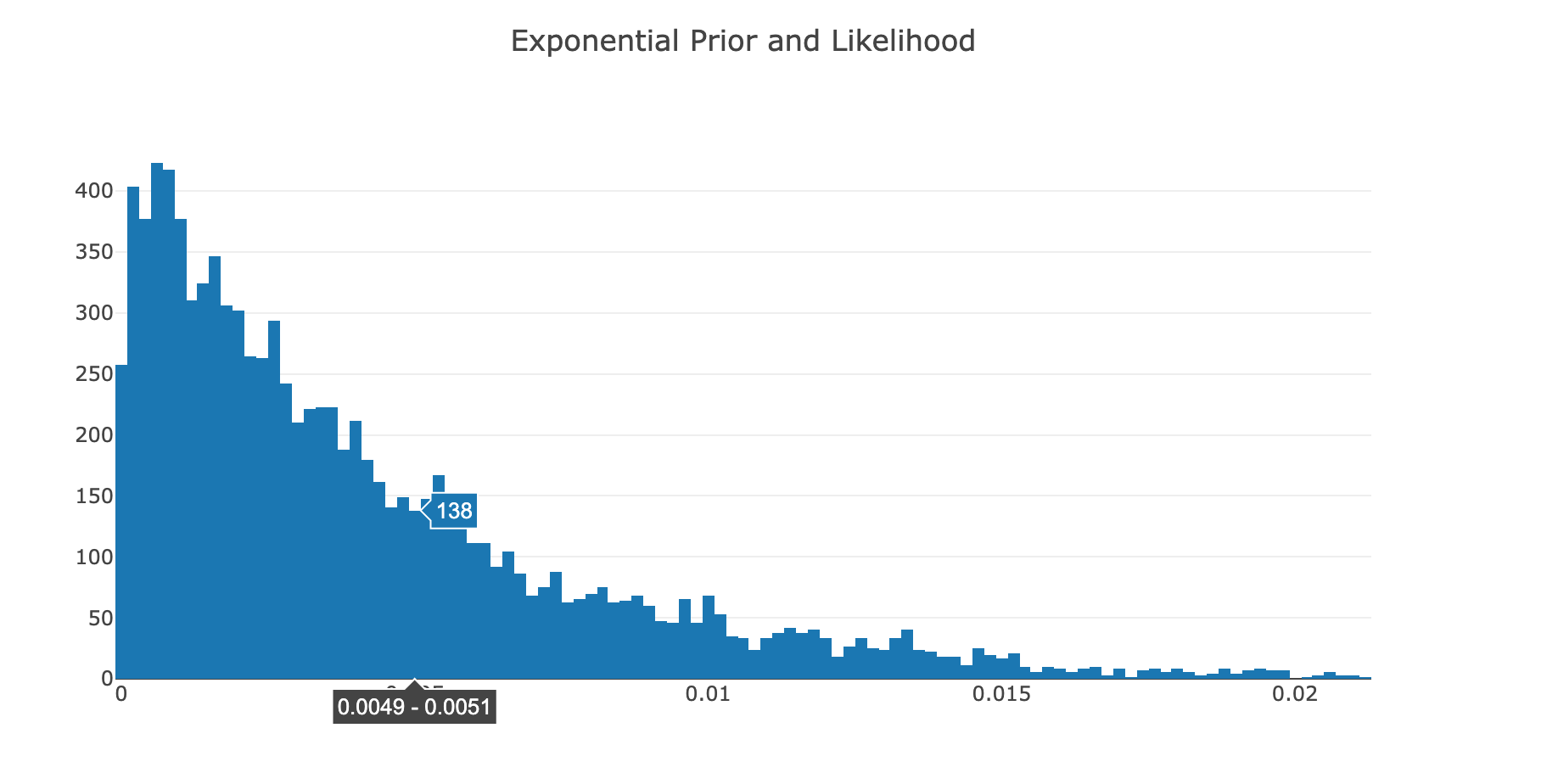
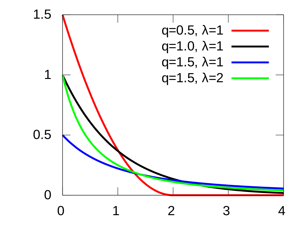
This histogram of the Step Values indicates that the Posterior has the shape of an Exponential distribution; which is expected. As an example, here is the PDF of a typical exponential distribution:
Normal Prior and Exponential Likelihood
#!fsharp
let model = @"x ~ Normal(μ,τ)
y|x ~ Exponential(x) : observed"
let parsedModel = parseModel model
let paramList = "{Parameters: {μ : 5, τ : 3.1622, σ : 1}, observed : [9.37,10.18,9.16,11.60,10.33]}"
let simpleModel =
SimpleBayesianNetworkModel.Construct "Normal-Exponential" parsedModel (deserializeParameters paramList)
let request : MCMCRequest =
{ StepFunction = SymmetricMetropolisHastings (ProposalDistribution.PositiveContinuousUniform 0.003, 0.0001)
ConvergenceCriteria = IterativeConvergence 50000
BurnInIterationsPct = 0.2
PrintDebug = false
Chains = 4 }
let mcmc = runMCMC request simpleModel
let firstChain = Seq.head mcmc.Chains
Histogram(x = firstChain.StepValues)
|> Chart.Plot
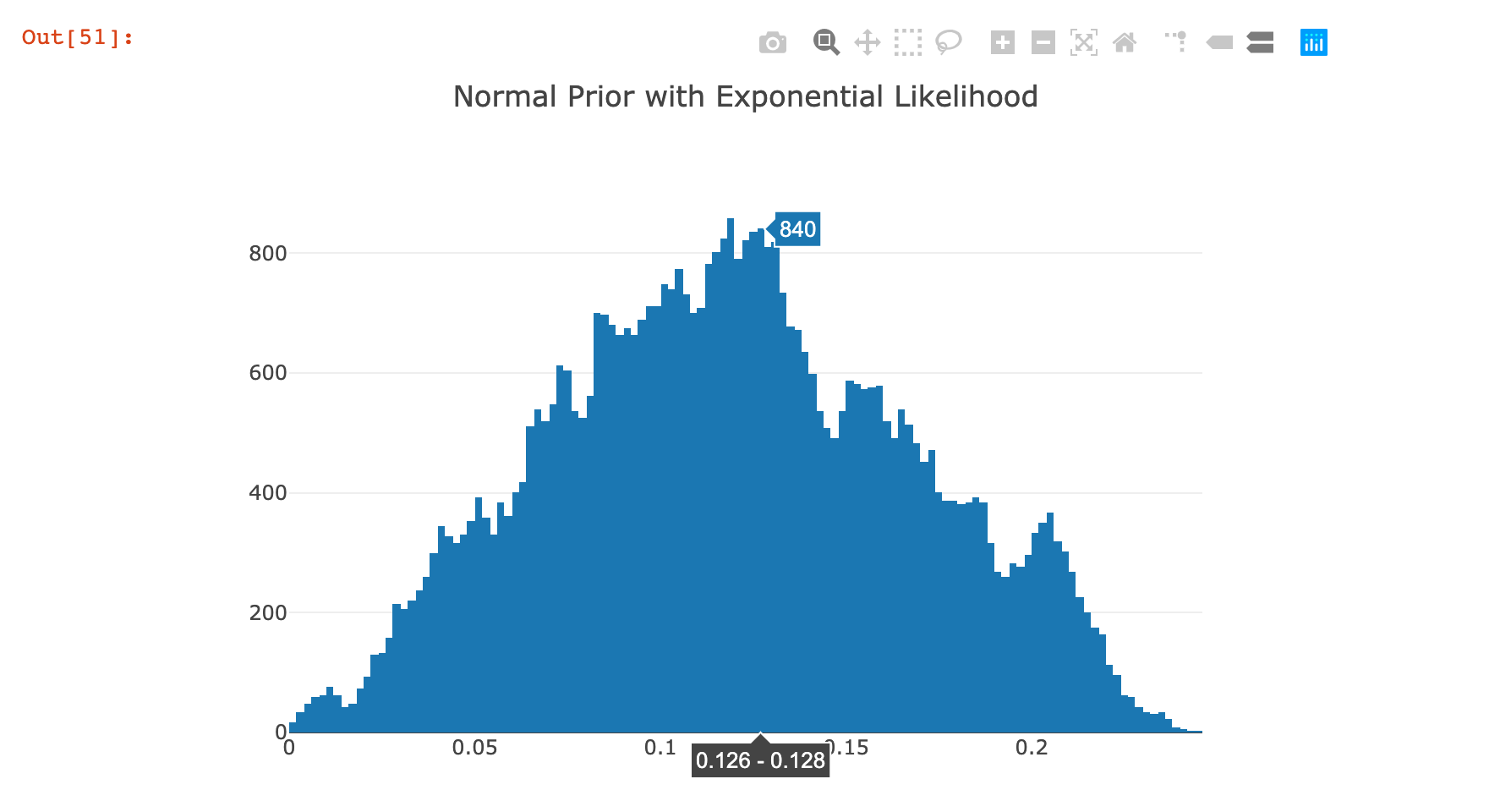
|> Chart.WithTitle "Normal Prior with Exponential Likelihood"
|> Chart.WithWidth 700
|> Chart.WithHeight 500
This posterior distribution was a lot more variable in terms of the shape of the distribution; it was also extremely dependent on the hyperparameters passed in highlighting the weaknesses of this algorithm. I am less confident about these results than those from the previous example.
How to Use the Posterior
Now that the posterior is obtained, the statistician could use it by sampling from it to plug in to other models used for prediction such as use it for the Posterior Predictive Distribution.
My plan is to write a separate blogpost to go over computing this and making use of the posterior to make predictions. This submission is already bloated enough.
Conclusion
This submission took a lot of work and is a product of two months of going down a Bayesian rabbit hole. Since I think I have built a reasonable base to continue to build on top of. As an obvious disclaimer, none of this code should be used in production - some of it is untested and might have bugs that weren't apparent to me while writing this.
Also, please let me know if you find any mistakes or can suggest any improvements! I'll be happy to learn from them and fix up this notebook.
Thanks to the organizers of FSharp-Advent and Happy Holidays to all!
Lessons and Prospective Improvements
Lessons
Debugging an Iterative Algorithm Can Be Challenging
Despite being a simple algorithm, the Symmetric Metropolis Hastings still has a lot of moving parts. Debugging through this was a big challenge! As much of cliche as it is, starting off small and passing in extremely simple parameters to complex algorithms was the way I debugged it. Also, adding optional print statements were helpful.
Tooling And Workflow is of Paramount Importance
Having the right workflow is extremely important for your productivity. I landed on making use of Jupyter notebooks with the .NET Interactive F# kernel. I briefly tried out the VSCode notebooks but got into issues such as inability to stop the kernel or cells running indefinitely. I will gladly assist with giving any feedback here as I think that feature has a lot of potential.
Prototyping Helps With Creating Modular Functions
I took a different approach with this submission than my previous one by first working on prototypical functions. I created a separate notebook where I wrote up all the functions / defined my domain and essentially prototyped the design. This was helpful as it gave me an opportunity to write and debug the algorithms productively.
Improvements
This Bayesian Rabbit hole I have got myself into is endless but unbelievably fun to understand. Here is how I envision improving the implementation and furthering my understanding of Bayesian Inference:
Better Parameter Parsing and Application
I dislike the current parameter parsing logic when mapping to distributions. I have currently hardcoded the parameter sequence i.e. the order in which parameters are passed in. In practice, a good Bayesian Inference library would introduce a more flexible way to specify a model.
More Generalized Bayesian Network
Right now, I have implemented a Simple Bayesian Network but want to generalize the implementation to a Generic Bayesian Network that'll work for all cases. Making use of a Directed Acyclic Graph (DAG) would be the way to represent this network and the computation of the joint distributions could be given by recursive equation that solves:
More Efficient MCMC Methods
As noted before, the Symmetric Metropolis Hastings algorithm has its flaws and there are more complex algorithms that give better results out there. I want to implement these from scratch. These include:
- Hamiltonian Monte-Carlo
- The No UTurn Sampler
- Gibbs Sampler with Metropolis Hastings for the Multivariate Case.
Branch out into Bayesian Regression
As a departure from the traditional Ordinary Least Squares Linear Regression algorithm, I want to venture into the space of Bayesian Regression that, in a nutshell, has regularization built into the algorithm.
Further Resources
Added to the Readme associated with this repository or here.
Recommend
About Joyk
Aggregate valuable and interesting links.
Joyk means Joy of geeK