Are you curious about artificial intelligence (AI) and machine learning (ML)? Do you want to know how to use it on the microcontrollers you already work with? In this article, we provide you with an introduction to ML on microcontrollers. This topic is also known as tiny machine learning (TinyML). Get ready for losing against an ESP-EYE at the rock, paper, scissors. You will learn about data collection and processing, how to design and train an AI and how to get it running on the MCU. This example provides you with all you need to do your own TinyML project from start to end.

Why Should I Care About TinyML?

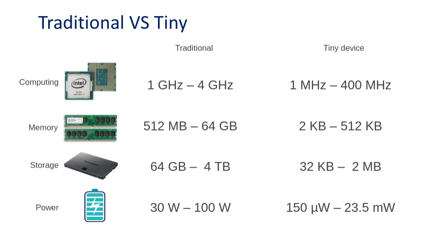
Surely you’ve heard of tech companies such as DeepMind and OpenAI. They dominate the ML domain with experts and GPU power. To give a sense of scale, the best AIs, such as those used by Google Translate, need months of training. They use hundreds of high-performance GPUs in parallel. TinyML turns the tables somewhat by going small. Because of memory limitations, large AI models don’t fit onto microcontrollers. The figure below shows the disparity between the hardware requirements.

What advantages does ML on MCUs offer over using AI services in the cloud? We find seven main strengths. 

1. Cost:Microcontrollers are cheap to buy and run.
2. Environmentally Friendly: Running AI on a microcontroller consumes little energy.
3. Integration: Microcontrollers are easily integrated into existing environments, for example, production lines.
4. Privacy and Security:Data can be processed locally and on the device. Data doesn’t have to be sent through the internet.
5. Rapid Prototyping: TinyML enables you to develop proof-of-concept solutions in a short period of time.
6. Autonomous and Reliable: Tiny devices can be used anywhere, even when there is no infrastructure.
7. Real-Time: The data is processed on the microcontroller without latency. The only limitation is the processing speed of the MCU.

Rock, Paper, Scissors

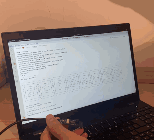
Have you ever lost the rock, paper, scissors against an AI? Or do you want to impress your friends by defeating an AI? You will play against an ESP-EYE board using TinyML. You need to learn five steps to make such a project possible. The following sections provide a high-level overview of the necessary steps. See the documentation in our project repository if you want to have a closer look. It explains the nifty details.

Gather Data

Collecting data is a crucial part of ML. To get things running, you need to take images of your hand forming a rock, paper, or scissors gesture. The more unique images the better. The AI will learn that your hand can be at different angles and positions or that lighting varies. A dataset contains the recorded images and, for each image, a label. This is known as supervised learning. 

It’s best to use the same sensors and environment for running your AI that were also used to train it. This will ensure that the model is familiar with the incoming data. For example, think of temperature sensors that have different voltage outputs for the same temperature due to manufacturing differences. For our purpose, this means that recording images with the ESP-EYE camera on a uniform background is ideal. During deployment, the AI will work best on a similar background. You could also record images with a webcam at the potential cost of some accuracy. Due to the limited capacity of the MCU, we record and process grayscale images of 96×96 pixels.

After collecting data, it’s important to split the data into a training and a test set. We do this to see how well our model recognizes images of hand gestures that it hasn’t seen before. The model will naturally do well on images that it has already seen during training.

Here are some example images. If you don’t want to collect data now, you can download our ready-made dataset here.

Preprocess Data

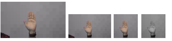
Recognizing patterns in data is not only hard for humans. To make this easier for an AI model, it’s common to rely on preprocessing algorithms. In our dataset, we recorded images using the ESP-EYE and a webcam. Since the ESP-EYE can capture grayscale images with 96×96 resolution, we don’t need much further processing here. However, we needed to downsize and crop the webcam images to 96×96 pixels and convert them from RGB to grayscale format. Lastly, we normalize all images. Below, you see the intermediate steps of our processing.

Design a Model

Designing a model is quite tricky! Detailed treatment is out of the scope of this article. We will describe the basic components of a model and how we designed ours. Under the hood, our AI relies on a neural network. You can think of a neural network as a collection of neurons, a bit like in our brains. That’s why in the case of a zombie apocalypse, AI would be eaten by Zombies, too.

When all neurons in a network are connected to each other, this is called fully connected or dense. This can be considered the most basic type of neural network. Since we would like our AI to recognize hand gestures from images, we use something a bit more advanced and suited for images, known as a convolutional neural network (CNN). Convolutions reduce the dimensionality of images, extract important patterns and preserve local relationships between pixels. To design a model, we use the TensorFlow library, which provides ready-made neural network components, called layers, that make creating neural networks easy!

Creating a model means stacking layers. The right combination of them is crucial to develop a robust and high-accuracy model. The figure below shows the different layers that we are using. Conv2D represents a convolutional layer. The BatchNormalization layer applies a form of normalization to the output of the layer above. Then we feed the data into the activation layer, which introduces non-linearity and filters out unimportant data points. Next, maximum pooling reduces the size of an image, similar to convolution. This block of layers is repeated a few times; the right amount is determined by experience and experimentation. After that, we use the flattening layer to reduce the two-dimensional images to a one-dimensional array. Lastly, the array is densely connected to three neurons which represent the classes rock, paper, and scissors.

def make_model_simple_cnn(INPUT_IMG_SHAPE, num_classes=3):
    inputs = keras.Input(shape=INPUT_IMG_SHAPE)
    x = inputs

    x = layers.Rescaling(1.0 / 255)(x)
    x = layers.Conv2D(16, 3, strides=3, padding="same")(x)
    x = layers.BatchNormalization()(x)
    x = layers.Activation("relu")(x)
    x = layers.MaxPooling2D()(x)
    x = layers.Conv2D(32, 3, strides=2, padding="same", activation="relu")(x)
    x = layers.MaxPooling2D()(x)
    x = layers.Conv2D(64, 3, padding="same", activation="relu")(x)
    x = layers.MaxPooling2D()(x)
    x = layers.Flatten()(x)
    x = layers.Dropout(0.5)(x)


    outputs = layers.Dense(units=num_classes, activation="softmax")(x)
    return keras.Model(inputs, outputs)

Train a Model

Once we have designed a model, we are ready to train it. Initially, the AI model will make random predictions. A prediction is a probability connected to a label; in our case, that’s rock, paper, or scissors. Our AI tells us how likely it considers an image to be each label. Because the AI is guessing labels at the start, it will often get labels wrong. Training happens after the predicted label is compared to the real label. Prediction errors lead to updates between the neurons in the network. This form of learning is called gradient descent. Because we built our model in TensorFlow, training is as easy as one, two, or three. Below, you see what the output produced during training is —  the higher the accuracy (train set) and validation accuracy (test set), the better!

Epoch 1/6
480/480 [==============================] - 17s 34ms/step - loss: 0.4738 - accuracy: 0.6579 - val_loss: 0.3744 - val_accuracy: 0.8718
Epoch 2/6
216/480 [============>.................] - ETA: 7s - loss: 0.2753 - accuracy: 0.8436

During training, multiple problems can occur. The most common problem is overfitting. As the model is exposed to the same examples over and over, it will start memorizing the training data by heart instead of learning the underlying patterns. Surely, you remember from school that understanding is better than memorization! At some point, the accuracy of the train data may continue going up while the accuracy on the test set doesn’t. This is a clear indicator of overfitting.

Convert a Model

After training, we obtain an AI model in the TensorFlow format. Because the ESP-EYE cannot interpret this format, we change the model into a microprocessor-readable format. We start with the conversion into a TfLite model. TfLite is a more compact TensorFlow format, which causes the model to decrease in size using quantization. TfLite is commonly used in edge devices, such as smartphones or tablets, all around the world. The last step is to convert the TfLite model to a C array, as the microcontroller is not capable of interpreting TfLite directly.

Deploy Model

Now we can deploy our model onto the microprocessor. The only thing we need to do is to place the new C array into the intended file. Replace the content of the C array, and don't forget to replace the array length variable at the end of the file. We’ve provided a script to make this easier. And that's it!

Embedded Environment

Let’s go over what happens in the MCU. During setup, the interpreter is configured to the shape of our images.

// initialize interpreter


static tflite::MicroInterpreter static_interpreter(
    model, resolver, tensor_arena, kTensorArenaSize, error_reporter);
interpreter = &static_interpreter;
model_input = interpreter->input(0);
model_output = interpreter->output(0);

// assert real input matches expect input
if ((model_input->dims->size != 4) || // tensor of shape (1, 96, 96, 1) has dim 4
    (model_input->dims->data[0] != 1) || // 1 img per batch
    (model_input->dims->data[1] != 96) || // 96 x pixels
    (model_input->dims->data[2] != 96) || // 96 y pixels
    (model_input->dims->data[3] != 1) || // 1 channel (grayscale)
    (model_input->type != kTfLiteFloat32)) { // type of a single data point, here a pixel
        error_reporter->Report("Bad input tensor parameters in model\n");
        return;
}

After the setup is complete, captured images are sent to the model, where a prediction about gestures is made. 

// read image from camera into a 1-dimensional array
uint8_t img[dim1*dim2*dim3]
if (kTfLiteOk != GetImage(error_reporter, dim1, dim2, dim3, img)) {
   TF_LITE_REPORT_ERROR(error_reporter, "Image capture failed.");
}

 // write image to model
 std::vector<uint8_t> img_vec(img, img + dim1*dim2*dim3);
 std::vector<float_t> img_float(img_vec.begin(), img_vec.end());
 std::copy(img_float.begin(), img_float.end(),  model_input->data.f);

 // apply inference
 TfLiteStatus invoke_status = interpreter->Invoke();
}

The model then returns a probability for each gesture. Since a probability array is only a series of values between zero and one, some interpretation is necessary. We consider the recognized gesture to be the one with the highest probability. Now we handle the interpretation by comparing the recognized gesture against the AI’s move and determine who won the round. You have no chance!

// probability for each class

float paper = model_output->data.f[0];

float rock = model_output->data.f[1];
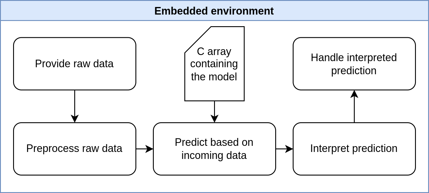
float scissors = model_output->data.f[2];

The cute diagram below illustrates the steps in the MCU. For our purposes, no preprocessing on the microcontroller is necessary.

Expand the Example

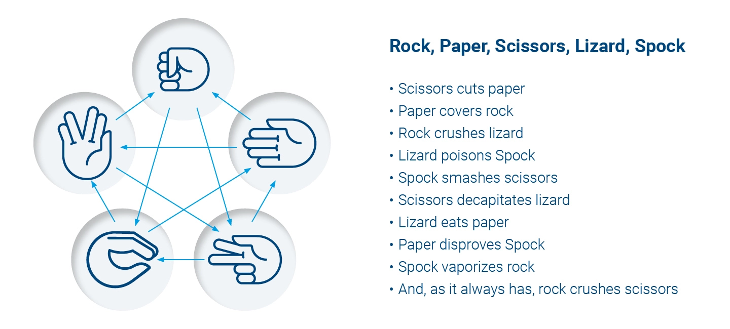
How about a challenge? A new purpose in life? Want to impress old friends or find new ones? Take a rock, paper, scissors to the next level by adding lizard and Spock. Your AI friend will be one skill closer to world domination. Well, first, you should have a look at our rock, paper, scissors repository and be able to replicate the steps above. The README files will help you with the details. The figure below shows you how the game works. You need to add two extra gestures and a few new winning and losing conditions.

Start Your Own Project

If you liked this article and want to start your own projects, we provide you with a template project which uses the same simple pipeline as our rock, paper, scissors project. You can find the template here. Don't hesitate to show us your projects via social media. We are curious to see what you are able to create!

You can find out more about TinyML here and there. Pete Warden’s book is a great resource.