Stable Diffusion’s latent space

Stable Diffusion uses three trained artificial neural networks in tandem:

The Variational Auto Encoder (VAE) encodes and decodes images from image space into some latent space representation. The latent space representation is a lower resolution (64 x 64), higher precision (4x32 bit) representation of any source image (512 x 512 at 3x8 or 4x8 bit).

How the VAE encodes the image into this latent space, it learns by itself during the training process and thus the latent space representations of different versions of the model will likely look different as the model gets trained further, but the representation of Stable Diffusion v1.4 looks like this (when remapped and interpreted as 4-channel color image):

The main features of the image are still visible when re-scaling and interpreting the latents as color values (with alpha channel), but the VAE also encodes the higher resolution features into these pixel values.

One encode/decode roundtrip through this VAE looks like this:

VAE roundtrip, from left to right: 512x512@24bpp ground truth, 64x64@128bpp latent space representation, 512x512@24bpp decoded image

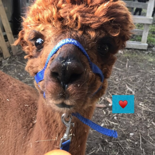
Note that this roundtrip is not lossless. For example, Anna’s name on her headcollar is slightly less readable after the decoding. The VAE of the 1.4 stable diffusion model is generally not very good at representing small text (as well as faces, something I hope version 1.5 of the trained model will improve).

The main algorithm of Stable Diffusion, which generates new images from short text descriptions, operates on this latent space representation of images. It starts with random noise in the latent space representation and then iteratively de-noises this latent space image by using the trained U-Net, which in simple terms outputs predictions of what it thinks it “sees” in that noise, similarly to how we sometimes see shapes and faces when looking at clouds. When Stable Diffusion is used to generate images, this iterative de-noising step is guided by the third ML model, the text encoder, which gives the U-Net information about what it should try to see in the noise. For the experimental image codec presented here, the text encoder is not needed. The Google Colab code shared below still makes use of it, but only to create a one-time encoding of an empty string, used to tell the U-Net to do un-guided de-noising during image reconstruction.

Compression Method

To use Stable Diffusion as an image compression codec, I investigated how the latent representation generated by the VAE could be efficiently compressed. Downsampling the latents or applying existing lossy image compression methods to the latents proved to massively degrade the reconstructed images in my experiments. However, I found that the VAE’s decoding seems to be vey robust to quantization of the latents.

Quantizing the latents from floating point to 8-bit unsigned integers by scaling, clamping and then remapping them results in only very little visible reconstruction error:

Left: decoded from 32-bit floating point latents — Middle: ground truth — Right: decoded from 8-bit integer latents

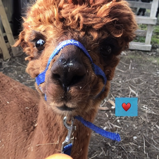
To quantize the latents generated by the VAE, I first scaled them by 1 / 0.18215, a number you may have come across in the Stable Diffusion source code already. It seems dividing the latents by this number maps them quite well to the [-1, 1] range, though some clamping will still occur.

By quantizing the latents to 8-bit, the data size of the image representation is now 64*64*4*8 bit = 16 kB (down from the 512*512*3*8 bit= 768 kB of the uncompressed ground truth)

Quantizing the latents to less than 8-bit didn’t yield good results in my experiments, but what did work surprisingly well was to further quantize by palettizing and dithering them. I created a palettized representation using a latent palette of 256 4*8-bit vectors and Floyd-Steinberg dithering. Using a palette with 256 entries allows to represent each latent vector using a single 8-bit index, bringing the data size to 64*64*8+256*4*8 bit = 5 kB

The palettized representation however now does result in some visible artifacts when decoding them with the VAE directly:

decoded from Left: 32-bit latents — Middle: 8-bit quantized latents — Right: palettized 8-bit latents with Floyd-Steinberg dithering (note the visible distortions)

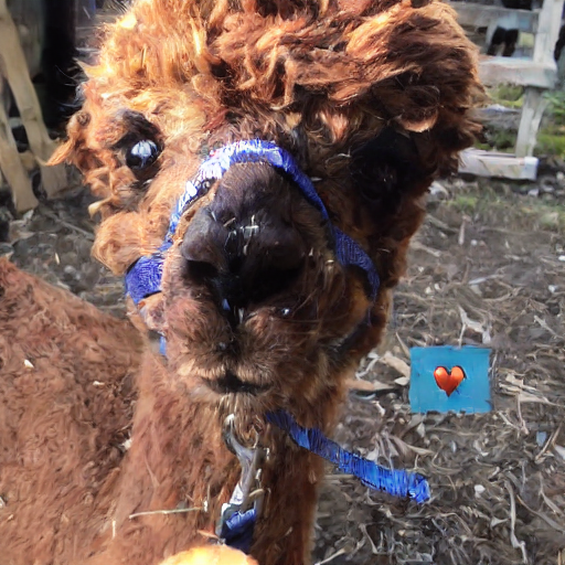
The dithering of the palettized latents has introduced noise, which distorts the decoded result. But since Stable Diffusion is based on de-noising of latents, we can use the U-Net to remove the noise introduced by the dithering. After just 4 iterations, the reconstruction result is visually very close to the unquantized version:

Left: after palettizing and dithering latents — Middle: after 4 de-noising steps — Right: Ground Truth

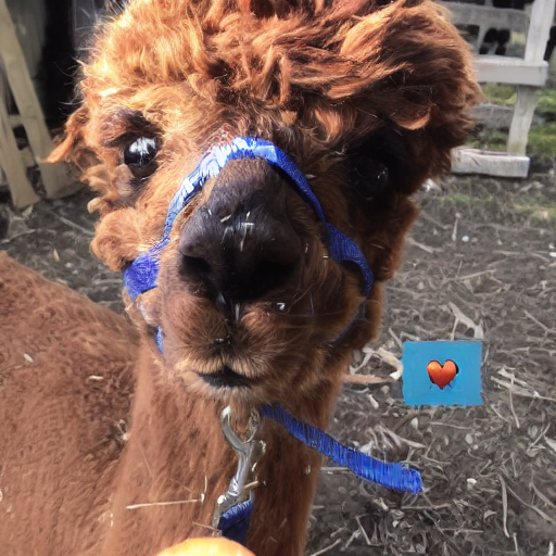
While the result is very good considering the extreme reduction in data size, one can also see though that artifacts got introduced, for example a glossy shade on the heart symbol that wasn’t present before compression. It’s interesting however how the artifacts introduced by this compression scheme are affecting the image content more so than the image quality, and it’s important to keep in mind that images compressed in such a way may contain these kinds of compression artifacts.

Finally, I losslessly compress the palette and indices using zlib, resulting in slightly under 5kB for most of the samples I tested on. I looked into run-length encoding, but the dithering leaves only very short runs of the same index for most images (even for those images which would work great for run-length encoding when compressed in image space, such as graphics without a lot of gradients). I’m pretty sure though there’s still even more optimization potential here to be explored in the future.

Evaluation

To evaluate this experimental compression codec, I didn’t use any of the standard test images or images found online in order to ensure that I’m not testing it on any data that might have been used in the training set of the Stable Diffusion model (because such images might get an unfair compression advantage, since part of their data might already be encoded in the trained model). Also, to make the comparison as fair as possible, I used the highest encoder quality settings for the JPG and WebP compressors of Python’s Image library and I additionally applied lossless compression of the compressed JPG data using the mozjpeg library. I then used the compression strength 1 less than what would result in a data size smaller than the Stable Diffusion result, or maximum strength otherwise (many images don’t get smaller than the SD result even at maximum lossy JPG or WebP compression).

It’s important to note that while the Stable Diffusion results look subjectively a lot better than the JPG and WebP compressed images, they are not significantly better (but neither worse) in terms of standard measurement metrics like PSNR or SSIM. It’s just that the kind of artifacts introduced are a lot less notable, since they affect image content more than image quality — which however is also a bit of a danger of this method: One must not be fooled by the quality of the reconstructed features — the content may be affected by compression artifacts, even if it looks very clear. for example, looking at a detail in the San Francisco test image:

Left: JPG compressed — Middle: Ground Truth — Right: Stable Diffusion Compressed

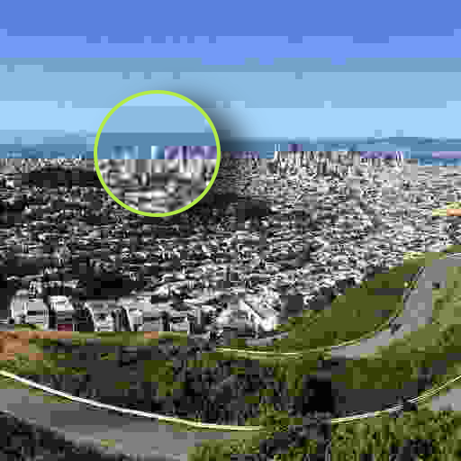
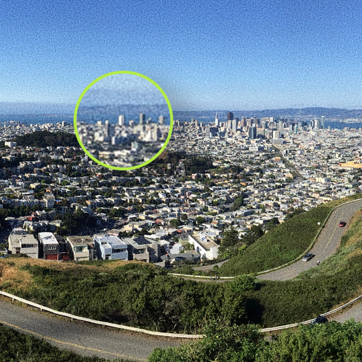
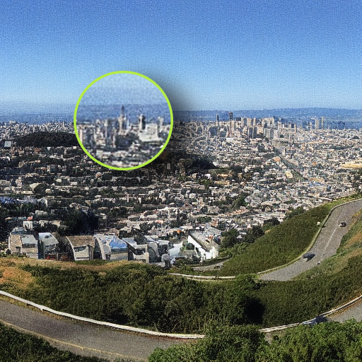
As you can see, while Stable Diffusion as codec is a lot better at preserving qualitative aspects of the image down to grain of the image (something that most traditional compression algorithms struggle with), the content is still affected by compression artifacts and as such fine features such as the shape of buildings may change and while it’s cetainly not possible to recognize more of the Ground Truth in the JPG compressed image than in the Stable Diffusion compressed image, the high quality of the SD result can be deceiving, since the compression artifacts in JPG and WebP are much more easily identified as such.