

论文解读(JKnet)《Representation Learning on Graphs with Jumping Knowledge Netw...
source link: https://www.cnblogs.com/BlairGrowing/p/16544425.html
Go to the source link to view the article. You can view the picture content, updated content and better typesetting reading experience. If the link is broken, please click the button below to view the snapshot at that time.

论文标题:Representation Learning on Graphs with Jumping Knowledge Networks
论文作者:Keyulu Xu, Chengtao Li, Yonglong Tian, Tomohiro Sonobe, Ken-ichi Kawarabayashi, Stefanie Jegelka
论文来源:2018,ICML
论文地址:download
论文代码:download
1 Introduction
关于多尺度信息的使用,本文的名字是 jumping knowledge (JK) networks。比较有意思的不是模型,而是将 “邻域聚合” 和 随机游走相对比,以及探索了中心节点 vv 受多层之后其他节点的影响。
2 Model analysis
除图属性信息很重要之外,图的结构对 “邻域聚合” 算法同样很重要。
同样一个图中,如果起点不同,random walk 相同步数之后的影响范围也就不同,random walk 多少步对应的就是卷积的迭代次数。
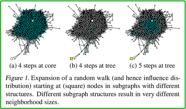
如上图所示,(a)、(b)、(c) 中 均以 square node 为起点。(a)中 square node 出现在中心稠密处 [core];(b)中出现在图边缘处【此时的 random walk 路径类似于树结构】;(c) 在 (b) 的基础上, random walk 的终点位于中心稠密处。
h(l+1)N(i)=aggregate({hlj,∀j∈N(i)})h(l+1)i=σ(W⋅concat(hli,hl+1N(i)))hN(i)(l+1)=aggregate({hjl,∀j∈N(i)})hi(l+1)=σ(W⋅concat(hil,hN(i)l+1))
→ 是否可以自适应地调整(即学习)每个节点的受影响半径?【可能 要减少 所谓 “邻域” 的大小】
→为实现这一点,本文探索了一种学习有选择地利用来自不同 “邻域” 的信息的架构,将表示“跳转”到最后一层。
3 Related work
3.1 neighborhood aggregation scheme
典型的邻域聚合方案如下:
h(l)v=σ(Wl⋅AGGREGATE({h(l−1)u,∀u∈N~(v)}))(1)hv(l)=σ(Wl⋅AGGREGATE({hu(l−1),∀u∈N~(v)}))(1)
3.2 Graph Convolutional Networks (GCN)
Recall
two-layer GCN :
Z=f(X,A)=softmax(A^ReLU(A^XW(0))W(1))Z=f(X,A)=softmax(A^ReLU(A^XW(0))W(1))
其中,A^=D~−12A~D~−12A^=D~−12A~D~−12
Kipf 提出的 GCN:
其中,cji=|N(j)|−−−−−√|N(i)|−−−−−√cji=|N(j)||N(i)|
h(l)v=ReLU(Wl⋅1deg(v)˜∑u∈N˜(v)h(l−1)u)hv(l)=ReLU(Wl⋅1deg(v)~∑u∈N~(v)hu(l−1))
显然就是,A^=D~−1A~(3)A^=D~−1A~(3)
GCN 的 inductive 变形:
hkv←σ(W⋅MEAN({hk−1v}∪{hk−1u,∀u∈N(v)}))hvk←σ(W⋅MEAN({hvk−1}∪{huk−1,∀u∈N(v)}))
3.3 Neighborhood Aggregation with Skip Connections
h(l)N(v)h(l)v=σ(Wl⋅AGGREGATEN({h(l−1)u,∀u∈N(v)}))=COMBINE(h(l−1)v,h(l)N(v))(4)hN(v)(l)=σ(Wl⋅AGGREGATEN({hu(l−1),∀u∈N(v)}))hv(l)=COMBINE(hv(l−1),hN(v)(l))(4)
COMBINE 步骤是这个范式的关键,可以被视为不同层之间的“skip connection”的一种形式。
GraphSAGE 的 Mean aggregator 形式:
hkv←σ(W⋅MEAN({hk−1v}∪{hk−1u,∀u∈N(v)})hkv←σ(Wk⋅CONCAT(hk−1v,hkN(v)))hvk←σ(W⋅MEAN({hvk−1}∪{huk−1,∀u∈N(v)})hvk←σ(Wk⋅CONCAT(hvk−1,hN(v)k))
3.4 Neighborhood Aggregation with Directional Biases
GAT、VAIN、 GraphSAGE 中的 max-pooling operation 修改了扩张的方向,而本文的模型则作用于扩张的局部性。
在第6节中,我们演示了我们的框架不仅适用于简单的邻域聚合模型(GCN),而且还适用于跳过连接(GraphSAGE)和 带 directional biase 的 GAT 。
4 Influence Distribution and Random Walks
受 sensitivity analysis 和 influence functions 的启发,我们研究了其特征影响给定节点表示的节点的范围,这个范围可以给出节点从中获取信息的邻域有多大。
本文测量节点 xx 对节点 yy 的敏感性,或者 yy 对 xx 的影响,通过测量 yy 的输入特征的变化对最后一层 xx 的表示的影响程度。对于任何节点 xx,influence distribution 捕获了所有其他节点的相对影响。
Definition 3.1 (Influence score and distribution). For a simple graph G=(V,E)G=(V,E) , let h(0)xhx(0) be the input feature and h(k)xhx(k) be the learned hidden feature of node x∈Vx∈V at the k−thk−th (last) layer of the model. The influence score I(x,y)I(x,y) of node xx by any node y∈Vy∈V is the sum of the absolute values of the entries of the Jacobian matrix [∂h(k)x∂h(0)y][∂hx(k)∂hy(0)] . We define the influence distribution IxIx of x∈Vx∈V by normalizing the influence scores: Ix(y)=I(x,y)/∑zI(x,z)Ix(y)=I(x,y)/∑zI(x,z) , or
Ix(y)=eT[∂h(k)x∂h(0)y]e/(∑z∈VeT[∂h(k)x∂h(0)z]e)Ix(y)=eT[∂hx(k)∂hy(0)]e/(∑z∈VeT[∂hx(k)∂hz(0)]e)
where ee is the all-ones vector.
对于 completeness ,我们还定义了 random walk distributions :
Definition 3.2. Consider a random walk on G˜G~ starting at a node v0v0 ; if at the t−tht−th step we are at a node vtvt , we move to any neighbor of vtvt (including vtvt ) with equal probability.The tt-step random walk distribution PtPt of v0v0 is
Pt(i)=Prob(vt=i)Pt(i)=Prob(vt=i)
随机游动分布的一个重要性质是,当 tt 的增加时,它变得更加扩散,如果图是非二部的,它收敛于极限分布。收敛速度取决于子图的结构,并且可以受随机游动跃迁矩阵的谱间隙的限制。
4.1 Model Analysis
以下结果表明,公共聚合方案的影响分布与随机游动分布密切相关。这一观察结果暗示了我们将讨论的具体含义——优势和缺点。
与 ReLU 激活的随机化假设类似,我们可以绘制GCNs和随机游动之间的联系:
Theorem 1. Given a kk-layer G C N with averaging as in Equation (3), assume that all paths in the computation graph of the model are activated with the same probability of success ρρ . Then the influence distribution IxIx for any node x∈Vx∈V is equivalent, in expectation, to the kk-step random walk distribution on G˜G~ starting at node xx .
证明如下:

通过修改 Theorem 1 的证明,可以直接证明 Eq.2Eq.2 中 GCN 版本的一个几乎等价的结果。
唯一的区别是每条从节点 x(v0p)x(vp0) 到 y(vkp)y(vpk) 随机行走的路径 v0p,v1p,…,vkpvp0,vp1,…,vpk 概率不是 ρ∏kl=11deg(vlp)¯¯¯¯¯¯¯¯¯¯¯¯¯¯¯¯¯¯ρ∏l=1k1deg(vpl)¯ ,而是 ρQ∏k−1l=11deg(vlp)˜⋅(deg˜(x)deg˜(y))−1/2ρQ∏l=1k−11deg(vpl)~⋅(deg~(x)deg~(y))−1/2,其中 QQ 是归一化因数。因此,概率上的差异很小,特别是当 xx 和 yy 的度很接近时。
同样地,我们可以证明具有方向性偏差的邻域聚集方案类似于有偏的随机游动分布。然后将相应的概率代入定理1的证明中。
根据经验,我们观察到,尽管有些简化的假设,我们的理论是接近于在实践中发生的事情。我们将训练过的gcn的一个节点(标记为平方)的影响分布的热图可视化,并与从同一节点开始的随机游动分布进行比较。Figure 2 显示了示例结果。
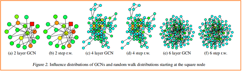
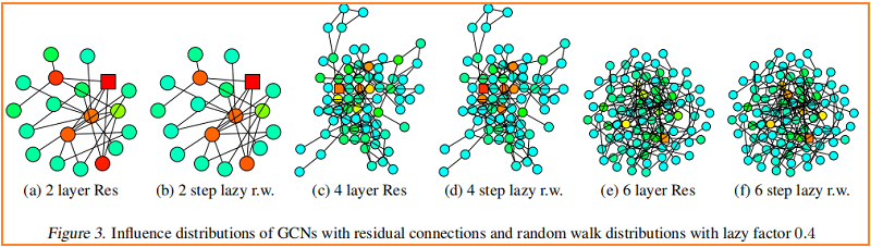
较深的颜色对应着较高的影响概率。为了显示跳过连接的效果,Figure 3 可视化了一个类似的热图——具有 residual connections 的 GCN。事实上,我们观察到,具有残差连接的网络的影响分布近似对应于惰性随机游动:每一步都有更高的概率停留在当前节点上。在每次迭代中,所有节点都以相似的概率保留局部信息;这不能适应特定上层节点的不同需求。
Fast Collapse on Expanders
从图中心开始的随机游走能在 O(log|V|)O(log|V|) 步骤中迅速收敛到一个几乎均匀的分布。在邻域聚合的 O(log|V|)O(log|V|) 迭代之后,通过 Theorem 1,每个节点的表示几乎受到图内部中任何其他节点的影响。因此,节点表示将代表全局图,并携带关于单个节点的有限信息。
相比之下,从 bounded tree-width 部分开始的随机游动收敛缓慢,即这些特征保留了更多的局部信息。施加固定随机游动分布的模型继承了这些扩展速度上的差异,并影响了邻域,这可能不会导致对所有节点的最佳表示
5 Jumping Knowledge Networks
大半径可能导致过多的平均,而小半径可能导致不稳定或信息聚集不足。因此,我们提出了两个简单而强大的架构变化——jump connection 和 subsequent selective 但自适应的聚合机制。
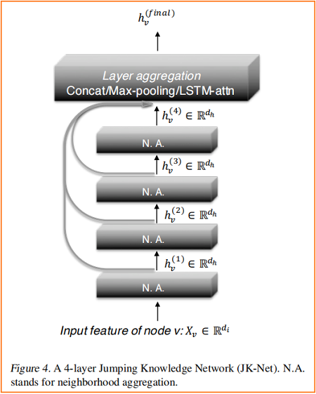
Figure 4 说明了主要的思想:在常见的邻域聚合网络中,每一层都通过聚集前一层的邻域来增加影响分布的大小。在最后一层,对于每个节点,我们仔细地从所有这些迭代表示(它们“跳转”到最后一层)中选择,潜在地结合一些。如果这是对每个节点独立完成的,那么该模型就可以根据需要调整每个节点的有效邻域大小,从而完全得到所需的自适应能力。
我们的模型允许一般的图层聚合机制。我们探索了三种方法;其他的也是可能的。设 h(1)v,…,h(k)vhv(1),…,hv(k) 是要聚合的节点 vv (来自 kk 个层)的跳跃表示。
Concatenation
h(1)i∥…∥h(T)ihi(1)‖…‖hi(T)
通常最后一层要加一个线性层。
JKNet(
  (dropout): Dropout(p=0.5, inplace=False)
  (layers): ModuleList(
    (0): GraphConv(in=1433, out=32, normalization=both, activation=<function relu>)
    (1): GraphConv(in=32, out=32, normalization=both, activation=<function relu>)
    (2): GraphConv(in=32, out=32, normalization=both, activation=<function relu>)
    (3): GraphConv(in=32, out=32, normalization=both, activation=<function relu>)
    (4): GraphConv(in=32, out=32, normalization=both, activation=<function relu>)
    (5): GraphConv(in=32, out=32, normalization=both, activation=<function relu>)
  )
  (jump): JumpingKnowledge()
  (output): Linear(in_features=192, out_features=7, bias=True)
)max(h(1)i,…,h(T)i)max(hi(1),…,hi(T))
优点:选择最具信息的特征,且不需要额外的参数
JKNet(
  (dropout): Dropout(p=0.5, inplace=False)
  (layers): ModuleList(
    (0): GraphConv(in=1433, out=32, normalization=both, activation=<function relu at 0x7f81d98fa550>)
    (1): GraphConv(in=32, out=32, normalization=both, activation=<function relu>)
    (2): GraphConv(in=32, out=32, normalization=both, activation=<function relu>)
    (3): GraphConv(in=32, out=32, normalization=both, activation=<function relu>)
    (4): GraphConv(in=32, out=32, normalization=both, activation=<function relu>)
    (5): GraphConv(in=32, out=32, normalization=both, activation=<function relu>)
  )
  (jump): JumpingKnowledge()
  (output): Linear(in_features=32, out_features=7, bias=True)
)
LSTM-attention
∑t=1Tα(t)ih(t)i∑t=1Tαi(t)hi(t)
输入 h(1)v,…,h(k)vhv(1),…,hv(k) 到 bi-directional LSTM ,并为每一层 ll 生成 forward-LSTM 和 backward-LSTM 隐藏特征 f(l)vfv(l) 和 b(l)vbv(l)。连接特征的线性映射 [f(l)v∥b(l)v][fv(l)‖bv(l)] 产生标量重要性分数 s(l)vsv(l)。对 {s(l)v}kl=1{sv(l)}l=1k 应用 Softmax 层求节点 vv 在不同层的注意力系数。使节点 vv 在不同范围内对其邻域的关注。最后,取 [f(l)v∥b(l)v][fv(l)‖bv(l)] 的和,用 SoftMax({s(l)v}kl=1)SoftMax({sv(l)}l=1k) 加权,得到最终的层表示。
JKNet(
  (dropout): Dropout(p=0.5, inplace=False)
  (layers): ModuleList(
    (0): GraphConv(in=1433, out=32, normalization=both, activation=<function relu>)
    (1): GraphConv(in=32, out=32, normalization=both, activation=<function relu>)
    (2): GraphConv(in=32, out=32, normalization=both, activation=<function relu>)
    (3): GraphConv(in=32, out=32, normalization=both, activation=<function relu>)
    (4): GraphConv(in=32, out=32, normalization=both, activation=<function relu>)
    (5): GraphConv(in=32, out=32, normalization=both, activation=<function relu>)
  )
  (jump): JumpingKnowledge(
    (lstm): LSTM(32, 80, batch_first=True, bidirectional=True)
    (att): Linear(in_features=160, out_features=1, bias=True)
  )
  (output): Linear(in_features=32, out_features=7, bias=True)
)
6 Experiments
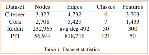
数据集
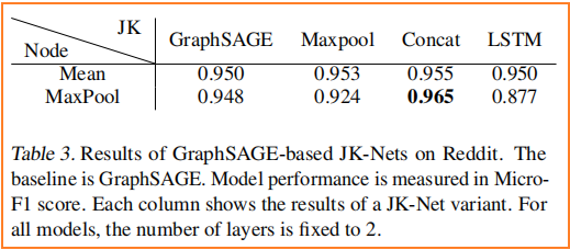
节点分类


7 Conclusion
__EOF__
Recommend
-
36
README.md AmpliGraph
-
47
On the Integration of Semantic Technologies and Symbolic Systems into Deep Learning Models for a More Comprehensible Artificial Intelligence
-
10
Helping the United Nations Infer Document Labels Using Knowledge Graphs
-
8
Machine Learning and Knowledge Graphs The Future of AI: Machine Learning and Knowledge Graphs Bringing knowledge graph and machine learning technology together can improve the accuracy of the outcomes and augmen...
-
6
On Knowledge Graphs and Grakn, with Daniel from Grakn LabsMarch 18th 2021 7
-
13
Technical Articles
-
5
【ICML 2018图神经网络论文解读】Representation Learning on Graphs with Jumping Knowledge Networks (JK-Net) 论文题目:Representation Learning on Graphs with Jumping Knowledge Networks 会...
-
11
论文解读(GRCCA)《 Graph Representation Learning via Contrasting Cluster Assignments》 论文标题:Graph Representation Learning via Contrasting Cluster Assignments论文作者:Chun-Yang Zhang, Hong-Yu Yao, C. L. Philip...
-
4
4 Dynamic Graph Representation Learning Via Self-Attention Networks link:https://arxiv.org/abs/1812.09430...
-
3
Note:[ wechat:Y466551 | 可加勿骚扰,付费咨询 ] 论文标题:Knowledge distillation for BERT unsupervised domain adaptation论文作者:Minho Ryu、Geonseok Lee、Kichun Lee论文来源:2022 aRxiv论文地址:
About Joyk
Aggregate valuable and interesting links.
Joyk means Joy of geeK