Find External Data for Machine Learning Pipelines

This article was published as a part of the Data Science Blogathon.

Introduction

Machine Learning pipelines are always about learning and best accuracy achievement. And every Data Scientist wants to progress as fast as possible, so time-saving tips & tricks are a big deal as well. That’s why low-code tools are adopted among data scientists. So, there are two major scenarios of external features & data introduction in the creation of machine learning pipelines for Data Scientists:

1. Final improvement of a polished machine learning pipelines

Use it to improve an already polished pipeline (optimized features, model architecture, hyperparameters) with new external features. And you want to answer the simple question – Are there any external data sources and features which might boost accuracy a bit more? However, there is a caveat to this approach: current model architecture & hyperparameters might be suboptimal for the new feature set, even a single new var after introduction. So extra step back for model tuning might be needed.

2. Low-code initial feature engineering – add relevant external features @start

Use it to save time on feature search and engineering. If there are some ready-to-use external features and data, let’s use them to speed up the overall progress. In this scenario always make sense to check that new external features have optimal representation for a specific task and target model architecture. Example – category features for linear regression models should be one-hot-encoded. This type of feature preparation should be done manually in any case. Same as scenario #1, there is a caveat to this approach: many features are not always a good thing – they might lead to dimensionality increase and model overfitting. So you have to check model accuracy improvement metrics after enrichment with the new features and ALWAYS with an appropriate cross-validation strategy.

In this guide, we’ll go with Scenario #1.

Let’s resolve such a task: TPS January 2022, SMAPE as a target metric.

And get the best open notebook for improvement.

To search for useful external data, we’ll use:

Upgini – Low-code Feature search and enrichment python library for supervised machine learning applications.

Packages

Let's install and import the packages that we will need.

%pip install -Uq upgini

import pandas as pd
import numpy as np
import pickle
import itertools
import gc
import math
import matplotlib.pyplot as plt
import dateutil.easter as easter
from datetime import datetime, date, timedelta
from sklearn.preprocessing import StandardScaler, MinMaxScaler
from sklearn.impute import SimpleImputer
from sklearn.model_selection import KFold, GroupKFold, TimeSeriesSplit
from sklearn.linear_model import Ridge
from sklearn.metrics import mean_squared_error
from sklearn.compose import ColumnTransformer
from sklearn.pipeline import make_pipeline
import lightgbm as lgb
import scipy.stats
import os

Python Code:

def generate_main_features(df):

    new_df = df[["row_id", "date", "country", "segment", "num_sold"]].copy()

    ## one-hot encoding

    new_df['Rama'] = df.store == 'Rama'

    for country in ['Finland', 'Norway']:

        new_df[country] = df.country == country

    for product in ['Mug', 'Hat']:

        new_df[product] = df['product'] == product
  

    ## datetime features

    new_df['wd4'] = np.where(df.date.dt.weekday == 4, 1, 0)

    new_df['wd56'] = np.where(df.date.dt.weekday >= 5, 1, 0)

    

    dayofyear = df.date.dt.dayofyear

    for k in range(1, 3):

        sink = np.sin(dayofyear / 365 * 2 * math.pi * k)

        cosk = np.cos(dayofyear / 365 * 2 * math.pi * k)

        new_df[f'mug_sin{k}'] = sink * new_df['Kaggle Mug']

        new_df[f'mug_cos{k}'] = cosk * new_df['Kaggle Mug']

        new_df[f'hat_sin{k}'] = sink * new_df['Kaggle Hat']

        new_df[f'hat_cos{k}'] = cosk * new_df['Kaggle Hat']

    new_df.drop(columns=['mug_sin1'], inplace=True)

    new_df.drop(columns=['mug_sin2'], inplace=True)

        

    # special days

    new_df = pd.concat([

        new_df,

        pd.DataFrame({f"dec{d}":(df.date.dt.month == 12) & (df.date.dt.day == d) for d in range(24, 32)}),

        pd.DataFrame({

            f"n-dec{d}": (df.date.dt.month == 12) & (df.date.dt.day == d) & (df.country == 'Norway') 

            for d in range(25, 32)

        }),

        pd.DataFrame({

            f"f-jan{d}": (df.date.dt.month == 1) & (df.date.dt.day == d) & (df.country == 'Finland')

            for d in range(1, 15)

        }),

        pd.DataFrame({

            f"n-jan{d}": (df.date.dt.month == 1) & (df.date.dt.day == d) & (df.country == 'Norway')

            for d in range(1, 10)

        }),

        pd.DataFrame({

            f"s-jan{d}": (df.date.dt.month == 1) & (df.date.dt.day == d) & (df.country == 'Sweden')

            for d in range(1, 15)

        })

    ], axis=1)

    

    # May and June

    new_df = pd.concat([

        new_df,

        pd.DataFrame({

            f"may{d}": (df.date.dt.month == 5) & (df.date.dt.day == d) 

            for d in list(range(1, 10))

        }),

        pd.DataFrame({

            f"may{d}": (df.date.dt.month == 5) & (df.date.dt.day == d) & (df.country == 'Norway')

            for d in list(range(18, 26)) + [27]

        }),

        pd.DataFrame({

            f"june{d}": (df.date.dt.month == 6) & (df.date.dt.day == d) & (df.country == 'Sweden')

            for d in list(range(8, 15))

        })

    ], axis=1)

    

    # Last Wednesday of June

    wed_june_map = {

        2015: pd.Timestamp(('2015-06-24')),

        2016: pd.Timestamp(('2016-06-29')),

        2017: pd.Timestamp(('2017-06-28')),

        2018: pd.Timestamp(('2018-06-27')),

        2019: pd.Timestamp(('2019-06-26'))

    }

    wed_june_date = df.date.dt.year.map(wed_june_map)

    new_df = pd.concat([

        new_df,

        pd.DataFrame({

            f"wed_june{d}": (df.date - wed_june_date == np.timedelta64(d, "D")) & (df.country != 'Norway')

            for d in list(range(-4, 5))

        })

    ], axis=1)

    

    # First Sunday of November

    sun_nov_map = {

        2015: pd.Timestamp(('2015-11-1')),

        2016: pd.Timestamp(('2016-11-6')),

        2017: pd.Timestamp(('2017-11-5')),

        2018: pd.Timestamp(('2018-11-4')),

        2019: pd.Timestamp(('2019-11-3'))

    }

    sun_nov_date = df.date.dt.year.map(sun_nov_map)

    new_df = pd.concat([

        new_df,

        pd.DataFrame({

            f"sun_nov{d}": (df.date - sun_nov_date == np.timedelta64(d, "D")) & (df.country != 'Norway')

            for d in list(range(0, 9))

        })

    ], axis=1)

    

    # First half of December (Independence Day of Finland, 6th of December)

    new_df = pd.concat([

        new_df,

        pd.DataFrame({

            f"dec{d}": (df.date.dt.month == 12) & (df.date.dt.day == d) & (df.country == 'Finland')

            for d in list(range(6, 15))

        }

    )], axis=1)




    # Easter

    easter_date = df.date.apply(lambda date: pd.Timestamp(easter.easter(date.year)))

    new_df = pd.concat([

        new_df,

        pd.DataFrame({

            f"easter{d}": (df.date - easter_date == np.timedelta64(d, "D"))

            for d in list(range(-2, 11)) + list(range(40, 48)) + list(range(51, 58))

        }),

        pd.DataFrame({

            f"n_easter{d}": (df.date - easter_date == np.timedelta64(d, "D")) & (df.country == 'Norway')

            for d in list(range(-3, 8)) + list(range(50, 61))

        })

    ], axis=1)

    

    features_list = [

        f for f in new_df.columns 

        if f not in ["row_id", "date", "segment", "country", "num_sold", "Rama"]

    ]

    return new_df, features_list




def get_gdp(row):

    country = 'GDP_' + row.country

    return gdp_df.loc[row.date.year, country]

        

def get_cci(row):

    country = row.country

    time = f"{row.date.year}-{row.date.month:02d}"

    if country == 'Norway': country = 'Finland'

    return cci_df.loc[country[:3].upper(), time].Value




def generate_extra_features(df, features_list):

    df['gdp'] = np.log(df.apply(get_gdp, axis=1))

    df['cci'] = df.apply(get_cci, axis=1)

    features_list_upd = features_list + ["gdp", "cci"]

    

    return df, features_list_upd

Final Improvement of Polished Pipeline

1. Let’s take an existing open solution with external data as a baseline

There are already external data in this solution, so improvement shouldn’t be an easy walk ;-):

1) GDP statistics per year/country (“gdp-20152019-finland-norway-and-sweden” dataset);
2) Consumer Confidence Index per year/month/country (Value field of “oecd-consumer-confidence-index” dataset).

And we want to improve the winning kernel by finding new/better external features.

There are no changes in feature engineering from the original notebook by @ambrosm.

So let’s calculate metrics for the baseline solution. First, read train/test data from csv, combine them in one dataframe and generate features:

input_data_path = "/input"
df, rama_ratio = read_main_data(input_data_path)
# a lot of calendar based features
df, baseline_features = generate_main_features(df)
print(df.shape)
print("Number of features:", len(baseline_features))
df.segment.value_counts()
# features from GDP and CCI
gdp_df, cci_df = read_additional_data(input_data_path)
df, top_solution_features = generate_extra_features(df, baseline_features)
print(df.shape)
set(top_solution_features) - set(baseline_features)

(32868, 172) Number of features: 166 (32868, 174)
{'cci', 'gdp'}

Define model, cross-validation split and apply cross-validation to estimate model accuracy:

model = Ridge(alpha=0.2, tol=0.00001, max_iter=10000)
cv = KFold(n_splits=5)

top_solution_scores, model_coef = cross_validate(model, df, top_solution_features, rama_ratio, cv=cv)
print("Top solution SMAPE by folds:", top_solution_scores)
print("Top solution avg SMAPE:", sum(top_solution_scores)/len(top_solution_scores))

Top solution SMAPE by folds: [4.239, 4.159, 4.168, 4.293, 4.077] 
Top solution avg SMAPE: 4.1872

Now, make the submission file:

submission_path = 'submission_top_solution.csv'
make_submission(model, df, top_solution_features, rama_ratio, submission_path)

The submission scores 4.13 on the public leaderboard and 4.55 on the private leaderboard (first place in the competition). This is our baseline.

Can we improve the first place solution even more? Let’s find out!

2. Find relevant external features

To find new features, we’ll use Upgini Feature search and enrichment library for supervised machine learning applications
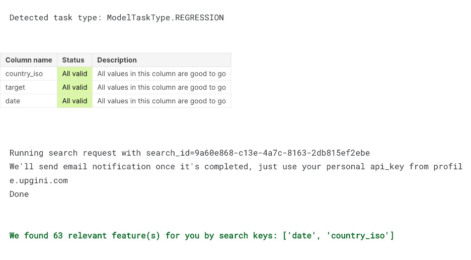
To initiate a search with the Upgini library, you must define so-called search keys – a set of columns to join external data sources. In this competition, we can use the following keys:

Column date should be used as SearchKey.DATE.;
Column country (after conversion to ISO-3166 country code) should be used as SearchKey.COUNTRY.

With this set of search keys, our dataset will be matched with different time-specific features (such as weather data, calendar data, financial data, etc.), considering the country where sales happened. Then relevant selection and ranking will be made. As a result, we’ll add new, only relevant features with additional information about specific dates and countries.

from upgini import SearchKey

# here we simply map each country to its ISO-3166 code
country_iso_map = {
    "Finland": "FI",
    "Norway": "NO",
    "Sweden": "SE"
}
df["country_iso"] = df.country.map(country_iso_map)

## define search keys
search_keys = {
    "date": SearchKey.DATE, 
    "country_iso": SearchKey.COUNTRY
}

To start the search, we need to initiate a scikit-learn compatible FeaturesEnricher transformer with appropriate search parameters. After that, we can call the fit method features_enricher to start the search.

The ratio between Rama and Mart sales is constant, so we’ll use only Mart sales for feature search and model training

%%time
from upgini import FeaturesEnricher
from upgini.metadata import CVType, RuntimeParameters

## define X_train / y_train, remove Mart
condition = (df.segment == "train") & (df.Rama == False)
X_train, y_train = df.loc[condition, list(search_keys.keys()) + top_solution_features], df.loc[condition, "num_sold"]

## define Features Enricher
features_enricher = FeaturesEnricher(
    search_keys = search_keys
)

CPU times: user 82 ms, sys: 14.7 ms, total: 96.7 ms Wall time: 4.59 s

FeaturesEnricher.fit() has a flag calculate_metrics For the quick estimation of quality improvement on cross-validation and eval sets. This step is quite similar to sklearn.model_selection.cross_val_score, so you can pass the exact metric with the scoring parameter:

Built-in scoring functions;
Custom scorer (in this case – scorer based on SMAPE loss).

And we pass the final Ridge model estimator with parameter, estimator for correct metric calculation, right in search results.
Notice that you should pass X_train as the first argument and y_train as the second argument for, FeaturesEnricher.fit(), just like in scikit-learn.

The step will take around 3.5 minutes

%%time
from sklearn.metrics import make_scorer

## define SMAPE custom scoring function
scorer = make_scorer(smape_loss, greater_is_better=False)
scorer.__name__ = "SMAPE"

## launch fit
features_enricher.fit(X_train, y_train,
                      calculate_metrics = True,
                      scoring = scorer,
                      estimator = model)

feature_name	shap_value	coverage %	type
0	Hat	0.507071	100.000000	NUMERIC
1	Mug	0.115800	100.000000	NUMERIC
2	f_cci_1y_shift_0fa85f6f	0.088312	66.666667	NUMERIC
3	mug_cos1	0.046179	100.000000	NUMERIC
4	f_pcpiham_wt_531b4347	0.029045	100.000000	NUMERIC
5	f_cci_6m_shift_653a5999	0.022123	66.666667	NUMERIC
6	f_year_sin1_16137bbf	0.019437	100.000000	NUMERIC
7	f_weekend_d0c2211b	0.014037	100.000000	NUMERIC
8	f_c2c_fraud_score_5028232e	0.010249	100.000000	NUMERIC
9	hat_sin1	0.010188	100.000000	NUMERIC
10	f_pcpihac_ix_16f52c8e	0.009000	100.000000	NUMERIC
11	f_credit_default_score_05229fa7	0.008933	100.000000	NUMERIC
12	f_weather_pca_0_94efd18d	0.007758	100.000000	NUMERIC
13	f_pcpih_wt_10c16d11	0.007703	100.000000	NUMERIC
14	Norway	0.007180	100.000000	NUMERIC
15	wd56	0.006366	100.000000	NUMERIC
16	f_pcpihah_ix_260dd0c8	0.006058	100.000000	NUMERIC
17	f_payment_fraud_score_3cae9c42	0.005449	100.000000	NUMERIC
18	f_cci_diff_1m_shift_fa99295c	0.004708	66.666667	NUMERIC
19	f_transaction_fraud_union_score_f9bc093c	0.003007	100.000000	NUMERIC
20	f_cci_pca_8_b72fe9f6	0.002578	100.000000	NUMERIC
21	f_holiday_public_7d_before_e3186344	0.002564	100.000000	NUMERIC
22	f_pcpih_ix_c2a9fea0	0.002472	100.000000	NUMERIC
23	f_days_to_election_e6b7c247	0.002158	100.000000	NUMERIC
24	f_pcpir_pc_cp_a_pt_3c2d5a5f	0.001977	100.000000	NUMERIC
25	f_holiday_national_7d_before_5ca8fb46	0.001935	100.000000	NUMERIC
26	f_pcpihabt_pc_cp_a_pt_41878919	0.001789	100.000000	NUMERIC
27	f_pcpihao_pc_cp_a_pt_0c75e62a	0.001649	100.000000	NUMERIC
28	mug_cos2	0.001381	100.000000	NUMERIC
29	f_cci_1m_shift_8b298796	0.001263	66.666667	NUMERIC
30	f_days_from_election_e1441706	0.001253	100.000000	NUMERIC
31	f_pcpi_pc_cp_a_pt_c1d5fdeb	0.001235	100.000000	NUMERIC
32	f_gold_7d_to_1y_1df66550	0.001215	100.000000	NUMERIC
33	f_holiday_code_7d_before_34f02a4f	0.001169	100.000000	NUMERIC
34	f_pcpifbt_ix_466ad65e	0.001150	100.000000	NUMERIC
35	f_holiday_bank_7d_before_efe82fb3	0.001147	100.000000	NUMERIC
36	f_pcpiec_ix_5dc7bc66	0.001098	100.000000	NUMERIC
37	f_cci_diff_6m_shift_52eb4cfe	0.001090	66.666667	NUMERIC
38	f_pcpied_pc_pp_pt_07be13cf	0.001085	100.000000	NUMERIC
39	f_pcpihah_wt_aad13a53	0.001043	100.000000	NUMERIC
40	f_PCPIEPCH_47b21aec	0.001013	100.000000	NUMERIC
41	f_year_sin2_46dc3051	0.000979	100.000000	NUMERIC
42	f_pcpio_ix_e60d7742	0.000933	100.000000	NUMERIC
43	f_year_cos1_cd165f8c	0.000922	100.000000	NUMERIC
44	f_pcpif_pc_cp_a_pt_507a914e	0.000915	100.000000	NUMERIC
45	gdp	0.000882	100.000000	NUMERIC
46	f_pcpir_ix_90fbe7c2	0.000867	100.000000	NUMERIC
47	Finland	0.000851	100.000000	NUMERIC
48	f_year_sin10_927d1cbc	0.000821	100.000000	NUMERIC
49	f_pcpihat_pc_cp_a_pt_803f3022	0.000787	100.000000	NUMERIC
50	f_days_to_holiday_5ce1a653	0.000755	100.000000	NUMERIC
51	f_cpi_pca_6_00674469	0.000713	100.000000	NUMERIC
52	f_year_cos2_2d8bf75c	0.000683	100.000000	NUMERIC
53	f_week_sin1_a71d22f6	0.000673	100.000000	NUMERIC
54	f_days_from_holiday_fbad7b66	0.000658	100.000000	NUMERIC
55	f_BCA_1y_shift_bcc8c904	0.000637	100.000000	NUMERIC
56	f_us_days_from_election_1658c931	0.000611	100.000000	NUMERIC
57	f_cpi_pca_2_3c36cd6c	0.000597	100.000000	NUMERIC
58	f_usd_eb23e09d	0.000591	100.000000	NUMERIC
59	f_dow_jones_89547e1d	0.000578	100.000000	NUMERIC

We’ve got 60+ relevant features, which might improve the model’s accuracy. Ranked by SHAP values.

Initial features from the search dataset will also be checked for relevancy, so you don’t need an extra feature selection step.

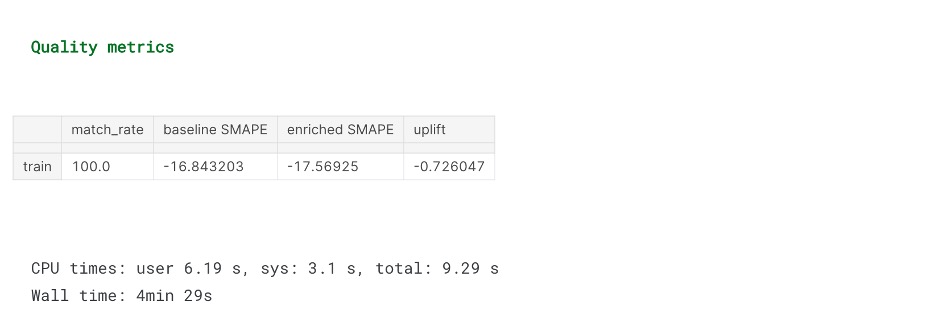
SMAPE uplift after enrichment with all of the new external features is negative – as it doesn’t make sense to use ALL of them for the linear Ridge model.

Let’s enrich the initial feature space with only the TOP-3 most important features.

Generally, it’s a bad idea to put a lot of features with unknown structure (and possibly high pairwise correlation) into a linear model, like Ridge or Lasso without careful selection and pre-processing.

The step will take around 2 minutes

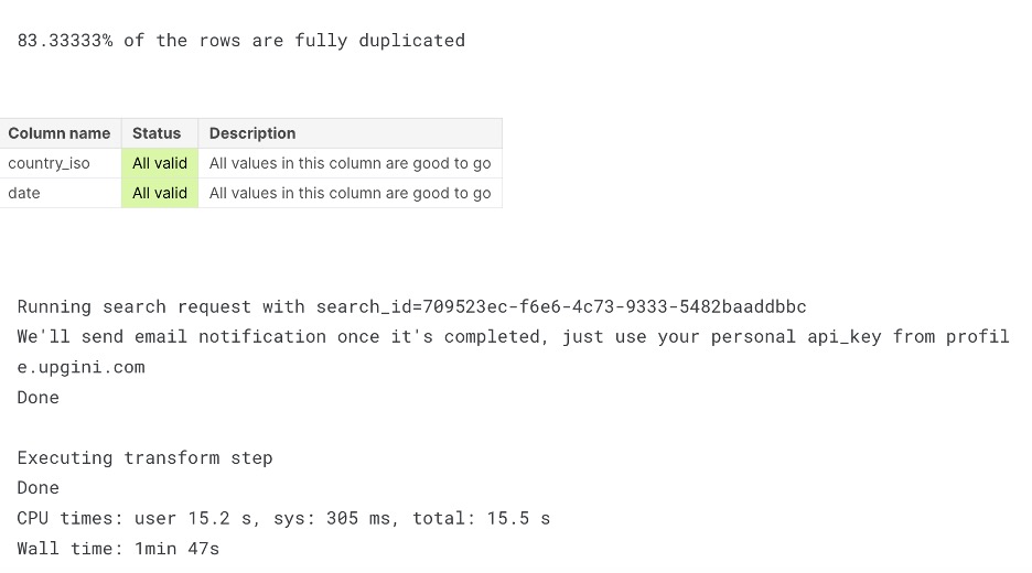
%%time

## call transform and enrich dataset with TOP-3 features only
df_enriched = features_enricher.transform(df, max_features=3, keep_input = True)

## put top-3 new external features names into selected features list
enricher_features = [
    f for f in features_enricher.get_features_info().feature_name.values
    if f not in list(search_keys.keys()) + top_solution_features
]
best_enricher_features = enricher_features[:3]

3. Submit and calculate the final leaderboard progress

Let’s estimate model quality and make a submission file:

#same cross-validation split and model estimator as for baseline notebook in #1 Part
upgini_scores, model_coef = cross_validate(
    model, df_enriched, 
    top_solution_features + best_enricher_features, 
    rama_ratio, cv=cv
)
print("Top solution SMAPE by folds:", top_solution_scores)
print("Upgini SMAPE by folds:", upgini_scores)
print("Top solution avg SMAPE:", sum(top_solution_scores)/len(top_solution_scores))
print("Upgini avg SMAPE:", sum(upgini_scores)/len(upgini_scores))

Top solution SMAPE by folds: [4.239, 4.159, 4.168, 4.293, 4.077]
Upgini SMAPE by folds: [4.26, 4.129, 4.144, 4.258, 4.051]
Top solution avg SMAPE: 4.1872
Upgini avg SMAPE: 4.1684

Make a submission file:

submission_path = 'submission.csv'
make_submission(
    model, df_enriched, 
    top_solution_features + best_enricher_features, 
    rama_ratio, submission_path)

This submission scores 4.095 on public LB and 4.50 on private LB.

Just to remind you – the baseline TOP-1 solution had 4.13 on public LB and 4.55 on private LB (with 2 external data sources already).
We’ve got a consistent improvement both in public and private parts of LB!

Relevant External Features & Data Sources

Leader board accuracy improved from enrichment with 3 new external features:

f_cci_1y_shift_0fa85f6f – Consumer Confidence Index with 1 year lag. It’s a Consumer Confidence Index value derivative for Finland and Sweden (CCI is unavailable for Norway). CCI as a feature already has been introduced in the baseline notebook, but as a raw CCI index value with scaling on the data prep step.
f_pcpiham_wt_531b4347 – Consumer Price index for Health group of products & services. In general, Consumer price indexes are index numbers that measure changes in the prices of goods and services purchased or otherwise acquired by households, which households use directly or indirectly to satisfy their needs and wants.
So it has a lot of information about inflation in a specific country and for a specific types of services and goods.
It’s been updated by the Organisation for Economic Cooperation and Development (OECD) every month.
f_cci_6m_shift_653a5999 – Consumer Confidence Index with 6 months lag.

Conclusion

When solving machine learning pipelines task, many data scientists forget that accuracy can be improved by implementing useful external data. Searching for external data can make the accuracy of your machine learning pipeline better, more accurate, and thus make you more money. I showed you how to find useful external data for minutes in this article.

Key takeaways of the article:

The article contains a description with python code of the way of developing of machine learning model with the best accuracy;
After reading the article, one can easily improve its ML model with external data;
The article contains an example of the real syntax of using the upgini python library;
Moreover, there is a list of real external data contained in upgini database for ML models that helped to improve an existing solution for ML tasks.

I hope you liked my article on machine learning pipelines and if you have any feedback or concerns, share with me in the comments below.

The media shown in this article is not owned by Analytics Vidhya and is used at the Author’s discretion.

Introduction

Packages

Final Improvement of Polished Pipeline

1. Let’s take an existing open solution with external data as a baseline

2. Find relevant external features

3. Submit and calculate the final leaderboard progress

Relevant External Features & Data Sources

Conclusion

Recommend

GitHub - kubeflow/pipelines: Machine Learning Pipelines for Kubeflow

Building Data Pipelines Learning Number 01- Die Monolith Die

Netflix's Metaflow: Reproducible machine learning pipelines

Top 10 US Cities To Find a Job in AI and Machine Learning

Building Machine Learning Pipelines: Common Pitfalls

Data Testing for Machine Learning Pipelines Using Deepchecks, DagsHub, and GitHu...

Configuration Driven Machine Learning Pipelines

Machine Learning Pipelines: Why Adopted by Data Scientists?

How to Orchestrate Data for Machine Learning Pipelines

Machine learning for Java developers: Machine learning data pipelines

About Joyk