Getting into Low-Latency Gears with Apache Flink - Part One

18 May 2022 Jun Qin & Nico Kruber

Apache Flink is a stream processing framework well known for its low latency processing capabilities. It is generic and suitable for a wide range of use cases. As a Flink application developer or a cluster administrator, you need to find the right gear that is best for your application. In other words, you don’t want to be driving a luxury sports car while only using the first gear.

In this multi-part series, we will present a collection of low-latency techniques in Flink. Part one starts with types of latency in Flink and the way we measure the end-to-end latency, followed by a few techniques that optimize latency directly. Part two continues with a few more direct latency optimization techniques. Further parts of this series will cover techniques that improve latencies by optimizing throughput. For each optimization technique, we will clarify what it is, when to use it, and what to keep in mind when using it. We will also show experimental results to support our statements.

This series of blog posts is a write-up of our talk in Flink Forward Global 2021 and includes additional latency optimization techniques and details.

Latency

Types of latency

Latency can refer to different things. LatencyMarkers in Flink measure the time it takes for the markers to travel from each source operator to each downstream operator. As LatencyMarkers bypass user functions in operators, the measured latencies do not reflect the entire end-to-end latency but only a part of it. Flink also supports tracking the state access latency, which measures the response latency when state is read/written. One can also manually measure the time taken by some operators, or get this data with profilers. However, what users usually care about is the end-to-end latency, including the time spent in user-defined functions, in the stream processing framework, and when state is accessed. End-to-end latency is what we will focus on.

How we measure end-to-end latency

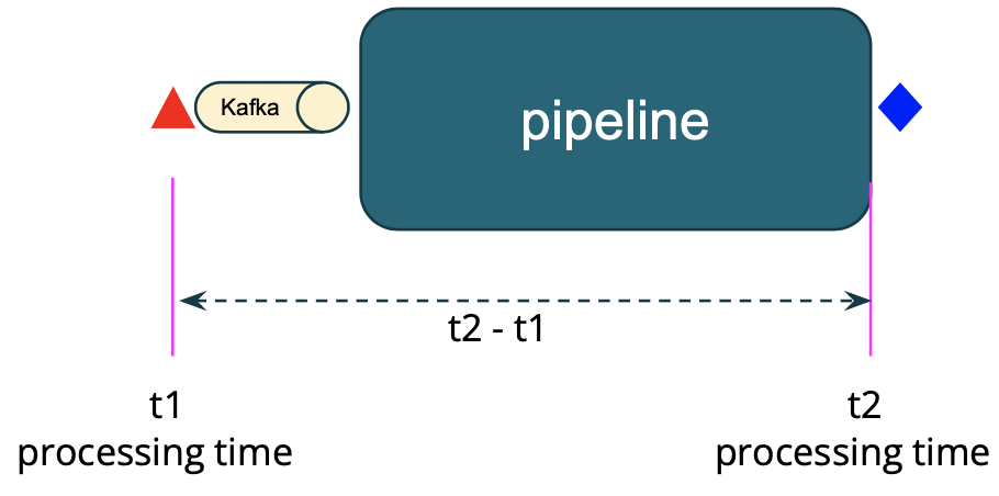
There are two scenarios to consider. In the first scenario, a pipeline does a simple transformation, and there are no timers or any other complex event time logic. For example, a pipeline that produces one output event for each input event. In this case, we measure the processing delay as the latency, that is, t2 - t1 as shown in the diagram.

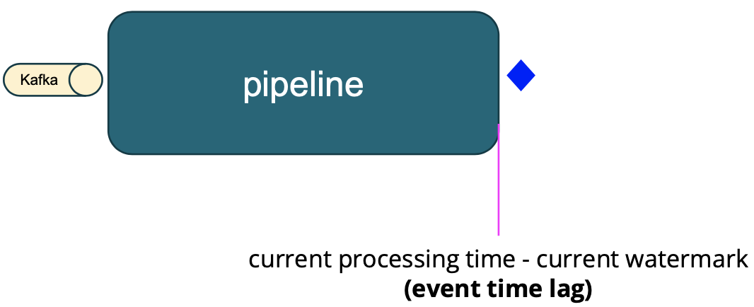
The second scenario is where complex event time logic is involved (e.g., timers, aggregation, windowing). In this case, we measure the event time lag as the latency, that is, current processing time - current watermark. The event time lag gives us the difference between the expected output time and the actual output time.

In both scenarios, we capture a histogram and show the 99th percentile of the end-to-end latency. The latency we measure here includes the time an event stays in the source message queue (e.g., Kafka). The reason for this is that it covers the scenarios where a source operator in a pipeline is backpressured by other operators. The more the source operator is backpressured, the longer the messages stay in the message queue. So, including the time events stay in the message queue in the latency gives us how slow or fast a pipeline is.

Low-latency optimization techniques

We will discuss low-latency techniques in two groups: techniques that optimize latency directly and techniques that improve latency by optimizing throughput. Each of these techniques can be as simple as a configuration change or may require code changes, or both. We have created a git repository containing the example jobs used in our experiments to support our statements. Keep in mind that all the experimental results we will show are specific to those jobs and the environment they run in. Your job may show different results depending on where the latency bottleneck is.

Direct latency optimization

Allocate enough resources

An obvious but often forgotten low-latency technique is to allocate enough resources to your job. Flink has some metrics (e.g., idleTimeMsPerSecond, busyTimeMsPerSecond, backPressureTimeMsPerSecond) to indicate whether an operator/subtask is busy or not. This can also be spotted easily in the job graph on Flink’s Web UI if you are using Flink 1.13 or later. If some operators in your job are 100% busy, they will backpressure upstream operators and the backpressure may propagate up to the source operators. Backpressure slows down the pipeline and results in high latency. If you scale up your job by adding more CPU/memory resources or scale out by increasing the parallelism, your job will be able to process events faster or process more events in parallel which leads to reduced latencies. We recommend having an average load below 70% under normal circumstances to accommodate load spikes that come from input data, timers, windowing, or other sources. You should adjust the threshold based on your job resource usage patterns and your latency requirements.

You can apply this optimization if your job or part of it is running at its total CPU/memory capacity and you have more resources that can be allocated to the job. In the case of scaling out with high parallelism, your streaming job must be able to make use of the additional resources. For example, the job should not have fixed parallelisms in the code, the job should not be bottlenecked on the source streams, and the input streams are partitionable by keys such that they can be processed in parallel and have no severe data skew, etc. In the case of scaling up by allocating more CPU cores, your streaming job must not be bottlenecked on a single thread or any other resources.

Keep in mind that allocating more resources may result in increased financial costs, especially when you are running jobs in the cloud.

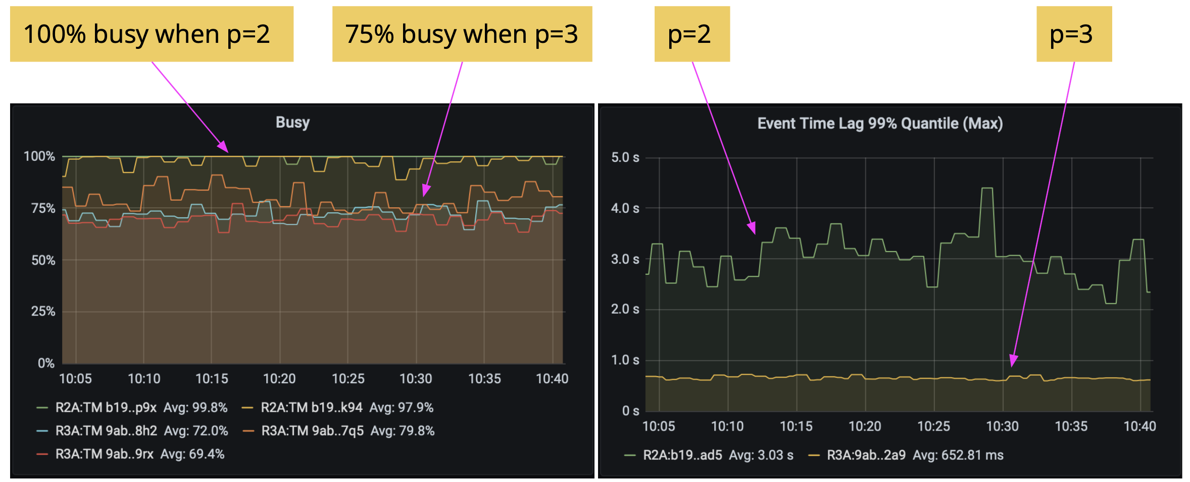
Below are the experimental results of WindowingJob. As you can see from the graph at the left, when the parallelism was 2, the two subtasks were often 100% busy. After we increased the parallelism to 3, the three subtasks were around 75% busy. As a result, the 99th percentile latency reduces from around 3 seconds to 650 milliseconds.

Use applicable state backends

When using the filesystem (Flink 1.12 or early) or hashmap (Flink 1.13 or later) state backend, the state objects are stored in memory and can be accessed directly. In contrast, when using the rocksdb state backend, every state access has to go through a (de-)serialization process which in addition may involve disk accesses. So using filesystem/hashmap state backend can help reduce latency.

You can apply this optimization if your state size is very small compared to the memory you can allocate to your job and your state size will not grow beyond your memory capacity. You can set the managed memory size to 0 if not needed. Since Flink 1.13, you can always start with the hashmap state backend and seamlessly switch to the rocksdb state backend via savepoints when the state increases to the size that is close to your memory capacity. Note that you should closely monitor the memory usage and perform the switch before an out-of-memory happens. Please refer to this Flink blog post for best practices when using the rocksdb state backend.

Keep in mind that heap-based state backends use more memory compared with RocksDB due to their copy-on-write data structure and Java’s on-heap object representation. Heap-based state backends can be affected by the garbage collector which makes them less predictable and may lead to high tail latencies. Also, as of now, there is no support for incremental checkpointing (this is being developed in FLIP-151). You should measure the difference before you make the switch.

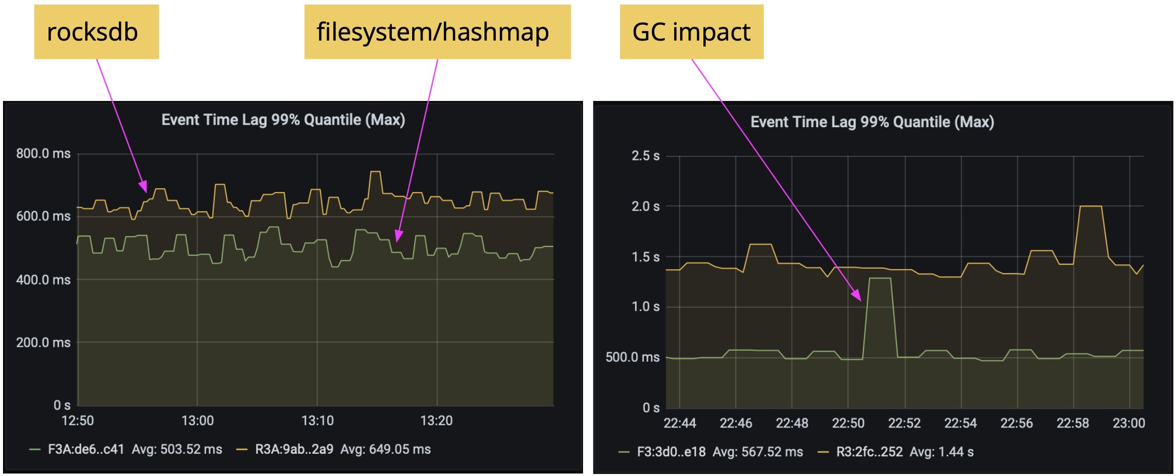
Our experiments with the previously mentioned WindowingJob after switching the state backend from rocksdb to hashmap show a further reduction of the latency down to 500ms. Depending on your job’s state access pattern, you may see larger or smaller improvements. The graph on the right shows the garbage collection’s impact on the latency.

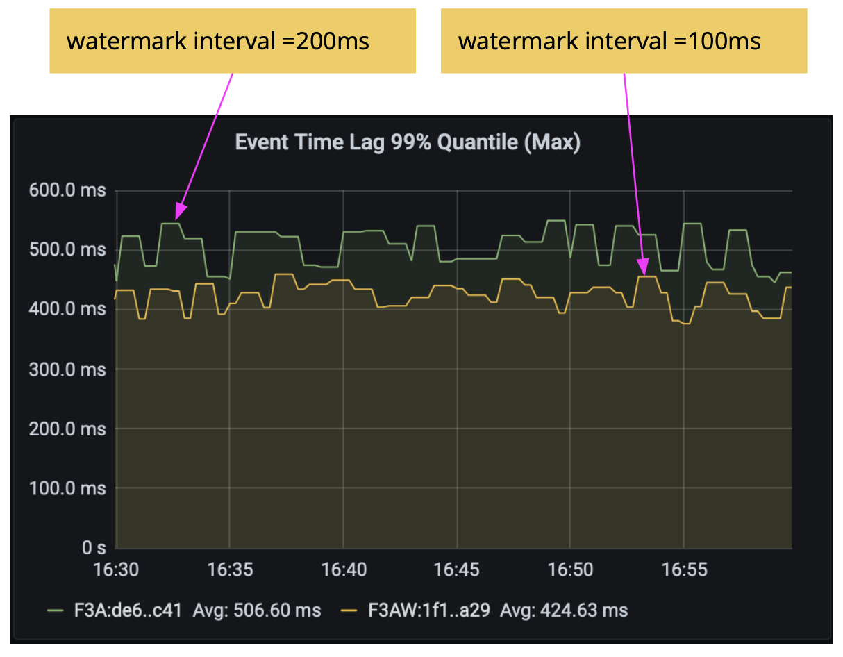
Emit watermarks quickly

When using a periodic watermark generator, Flink generates a watermark every 200 ms. This means that, by default, each parallel watermark generator does not produce watermark updates until 200 ms have passed. While this may be sufficient for many cases, if you are aiming for sub-second latencies, you could try reducing the interval even further, for example, to 100 ms.

You can apply this optimization if you use event time and a periodic watermark generator, and you are aiming for sub-second latencies.

Keep in mind that watermark generation that is too frequent may also degrade performance because more watermarks must be processed by the framework. Moreover, even though watermarks are only created every 200 milliseconds, watermarks may arrive at much higher frequencies further downstream in your job because tasks may receive watermarks from multiple parallel watermark generators.

We re-ran the previous WindowingJob experiment with the reduced watermark interval pipeline.auto-watermark-interval: 100ms and reduced the latency further to 430ms.

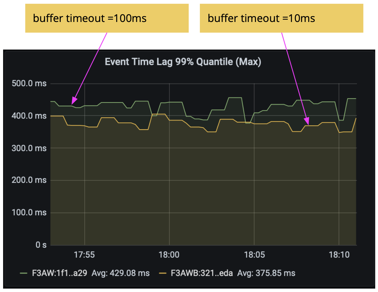
Flush network buffers early

Flink uses buffers when sending data from one task to another over the network. Buffers are flushed and sent out when they are filled up or when the default timeout of 100ms has passed. Again, if you are aiming for sub-second latencies, you can lower the timeout to reduce latencies.

You can apply this optimization if you are aiming for sub-second latencies.

Keep in mind that network buffer timeout that is too low may reduce throughput.

As seen in the following experiment results, by using execution.buffer-timeout: 10 ms in WindowingJob, we again reduced the latency (now to 370ms).

Summary

In part one of this multi-part series, we discussed types of latency in Flink and the way we measure end-to-end latency. Then we presented a few latency optimization techniques with a focus on direct latency optimization. For each technique, we explained what it is, when to use it, and what to keep in mind when using it. Part two will continue with a few more direct latency optimization techniques. Stay tuned!