

How to Create Stunning Dot Pattern Portraits, using Python
source link: https://numbersmithy.com/how-to-create-stunning-dot-pattern-portraits-using-python/
Go to the source link to view the article. You can view the picture content, updated content and better typesetting reading experience. If the link is broken, please click the button below to view the snapshot at that time.
How to Create Stunning Dot Pattern Portraits, using Python
This is a post inspired by a Photoshop tutorial on Youtube, entitled Photoshop: How to Create Stunning DOT Pattern Portraits!. In a nutshell, the tutorial illustrates how to use an array of colored disks to re-create a portrait photo, much like a pixelated art but using disks rather than squares. It is a fairly simple process (you can do that in minutes if you know Photoshop well), the effect is pretty stylistic (if not "stunning") and the tutorial itself is well presented. I recommend giving the video a watch if you are interested.
What I would like to do in this post is to mimic the dot pattern effect
as shown in that video, using not Photoshop, but Python tools.
More specifically, we will be using numpy for array data
manipulation, and opencv for image data read/write. The latter choice
is not crucial, you can replace that with other image file reading/writing
packages/modules as you like.
Below is the end result:
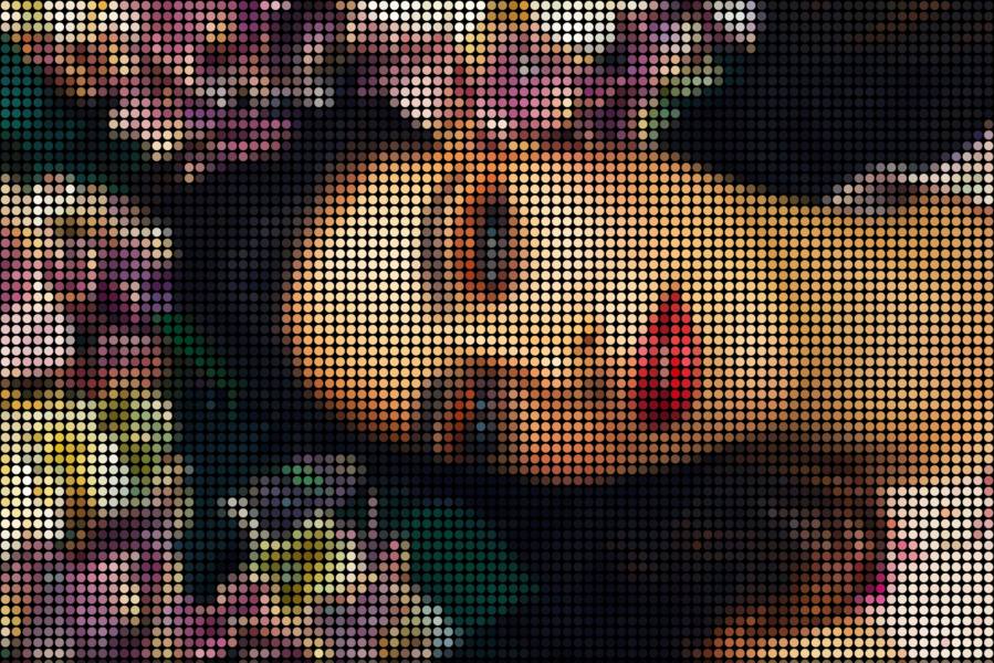
Figure 1. Final output of the dot pattern portrait.
Overview of the procedures
The procedures used in the tutorial video and in our implementation is summarized below:
0. Get a portrait photo
The Youtube tutorial used a very colorful portrait photo. To stick to the same flavor, I picked a royalty-free stock photo by Cihan Oğuzmetin from Pexels. Maybe not as color-saturated but it is good enough for the purpose of illustrating the technique. Figure 2 below shows a downgraded version of the photo (the original image has a pretty big 7360 x 4912 resolution).
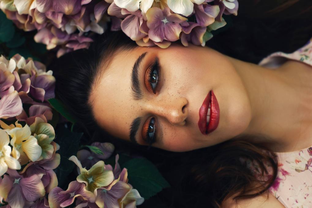
Figure 2. (Downgraded) portrait photo.
1. Pixelate the image
Pixelating an image can be achieved by the Pixelate -> Mosaic filter in Photoshop.
To view this process from an array number manipulation perspective, pixelating an image is to divide the image into a regular grid, coarser than the original resolution of cause, and replace the pixels in each grid cell with the average color value of the cell.
2. Create and apply a dot pattern/stencil
Inside Photoshop, a "pattern" is created from an ordinary image layer, usually in binary or gray scale, and can be used to fill up a region in canvas, or even used as brush shapes. In our dot pattern task, the "pattern" we are about to create is a filled disk (I think some mathematicians tend to be more sensitive about the distinctions between "circle" and "disk"), with a diameter the same as the length of the grid cell that we use to pixelate the image. So the effect is a pixel art made up with disks instead of squares.
In the field of image processing, the "pattern" idea is sometimes referred to as a "kernel", or a "structuring element", or a "stencil". I will be using the latter name here. Numerically, it is a 2D array with a smaller size than the image to be processed, and is used to perform some operations on the image, by sliding across the image in some manner. This may remind you of the convolution operation. In fact, I will be using some techniques introduced in a convolution related post to apply the stencil.
3. Add a line stroke on the dot stencil
In the Youtube tutorial, the tutor shrunk the dot patterns (the colored disks) by adding a 1-pixel line stroke on the interior side of the dot patterns.
We can achieve the same effect by shrinking the diameter of our disk stencil, to be slightly smaller than the grid cell length. It may sound a bit vogue now, but you will get the point when we implement it in code.
5. Enhance the color vibrancy and brightness of the image
So far we have been pretty much dealing with the dot pattern task from a geometrical perspective. Now we are moving onto the color territory. And to be honest I’m rather ignorant in this respect.
Maybe not just me, when searching about "how to enhance color vibrancy in Python" or similar questions, I didn’t get any clear-cut answer as I initially expected. I guess Photoshop being a close-source software is partly to blame, and also because how "vibrant" an image looks is somewhat a subjective judgment. So I’ll list the references I used when introducing the implementation details, but keep in mind that they may not the most accurate or suitable way of doing these.
Python implementation
Now let’s write some code.
One more thing to mention before we start:
I’m using opencv to read/write the image. Once read into Python,
images are represented as unsigned integers (unit8) with values from 0
to 255. Keep in mind that anything above 255 will trigger an
overflow, and as numpy arrays, this happens silently.
Read the image
import cv2

IMG_FILE = './dot_pattern.jpg'
image = cv2.imread(IMG_FILE)
print(f'{image.shape = }')

# BGR to RGB
image = image[:, :, ::-1]
Note that the last line changes the color channel from opencv‘s
BGR convention to a more commonly used RGB ordering. This is more
convenient for creating plots using, for instance, matplotlib, maybe
for debugging purposes.
But it is not crucial for our task, if you don’t want to make any
plots using matplotlib just ignore the last line.
Create dot patterns
First we create a disk stencil:
CELL = 80
MARGIN = 6

stencil = np.zeros([CELL, CELL]).astype('uint8')
yy, xx = np.mgrid[-CELL//2 : CELL//2, -CELL//2 : CELL//2]
stencil[(xx**2 + yy**2) <= (CELL//2 - MARGIN)**2] = 1
The diameter of the disk is defined as a constant 80.
Then we create a mesh grid, or a coordinate system, inside the 80 x 80 cell. The 0 point is at the center (strictly speaking one only gets the central row/column when the cell length is an odd number. But it’s not crucial in this case), and the disk is represented by points/pixels satisfying the equation:
where R is the radius of the disk, computed as CELL//2.
Figure 3a below shows our stencil.
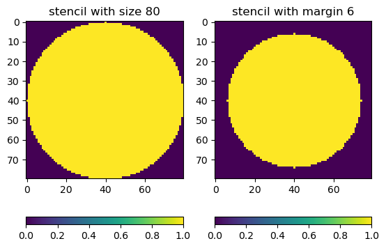
Figure 3. Left: Disk stencil with diameter 80. Right: Disk stencil with diameter 80 – 6.
The MARGIN parameter is used to add a gap between the disks such
that they don’t touch each other (see Figure 3b).
In the Youtube tutorial this was
achieved by adding a line stroke on the interior side of the disk
pattern.
Change the CELL and MARGIN values to your liking.
Pixelate the image
We need to divide the image into cells with size CELL.
The sizes of the image in general will not divide the cell size evenly, so we pad the image with 0s first:
def padArray(var, pad_y, pad_x):
    '''Pad array with 0s

    Args:
        var (ndarray): 2d or 3d ndarray. Padding is done on the first 2 dimensions.
        pad_y (int): number of rows to pad at bottom.
        pad_x (int): number of columns to pad at right.
    Returns:
        var_pad (ndarray): 2d or 3d ndarray with 0s padded along the first 2
            dimensions.
    '''
    if pad_y + pad_x == 0:
        return var

    var_pad = np.zeros((pad_y + var.shape[0], pad_x + var.shape[1]) + var.shape[2:])
    var_pad[:-pad_y, :-pad_x] = var

    return var_pad

# pad image size to the integer multiples of stencil
pad = padArray(image, CELL - image.shape[0] % CELL, CELL - image.shape[1] % CELL)
print(f'{pad.shape = }')
The output shape is:
pad.shape = (4960, 7440, 3)
Then we re-arrange the image into a new form that all the cells align
up. Imagine cutting the image up along the cell edges, and stacking all
the cell pieces vertically in a pile. This is achieved using the strided-view
trick of numpy, the same trick can be used to perform strided convolutions.
Here is the function that creates a strided-view from the image:
def asStride(arr, sub_shape, stride):
    '''Get a strided sub-matrices view of an ndarray.

    Args:
        arr (ndarray): input array of rank 2 or 3, with shape (m1, n1) or (m1, n1, c).
        sub_shape (tuple): window size: (m2, n2).
        stride (int): stride of windows in both y- and x- dimensions.
    Returns:
        subs (view): strided window view.

    See also skimage.util.shape.view_as_windows()
    '''
    s0, s1 = arr.strides[:2]
    m1, n1 = arr.shape[:2]
    m2, n2 = sub_shape[:2]

    view_shape = (1+(m1-m2)//stride, 1+(n1-n2)//stride, m2, n2)+arr.shape[2:]
    strides = (stride*s0, stride*s1, s0, s1)+arr.strides[2:]
    subs = np.lib.stride_tricks.as_strided(
        arr, view_shape, strides=strides, writeable=False)

    return subs
And below shows the application and the shape of the strided-view:
# create strided view of the padded image
pad_strided = asStride(pad, stencil.shape, CELL)
print(f'{pad_strided.shape = }')
pad_strided.shape = (62, 93, 80, 80, 3)
Notice that with a 80 x 80 cell size, our padded image has 62
rows and 93 columns, both measured in cell numbers.
Then to work out the mean value of each cell:
# pixelate image
cell_means = np.mean(pad_strided, axis=(2,3), keepdims=True)
print(f'{cell_means.shape = }')

pixelate = cell_means * np.ones(pad_strided.shape)
print(f'{pixelate.shape = }')
Here is the output:
cell_means.shape = (62, 93, 1, 1, 3)
pixelate.shape = (62, 93, 80, 80, 3)
Note that the image is now 5-dimensional. If we were to visualize the effect, we need to do some re-arrangements:
def stride2Image(strided, image_shape):
	res = strided.transpose([0, 2, 1, 3, 4])
	res = res.reshape(image_shape)
	return res

pixelate_img = stride2Image(pixelate, pad.shape)
pixelate_img = pixelate_img[:image.shape[0], :image.shape[1]]
The stride2Image() function reshapes the image into the normal
[Height, Width, Channel] format, and the last line crops out the
padded 0s.
Figure 4 below shows the effect of pixelation:
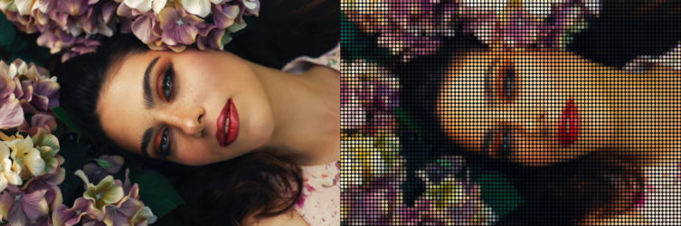
Figure 4. Compare the original image (left) with the pixelated version (right).
Apply the stencil
The stencil can be applied onto our strided-view directly:
# apply the dot stencil
filtered = pixelate * stencil[:, :, None]
print(f'{filtered.shape = }')
The output is
filtered.shape = (4912, 7360, 3).
Figure 5 below shows the effect (we are getting close):
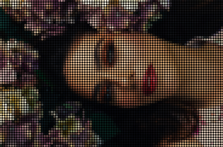
Figure 5. Apply dot pattern stencil.
Enhance colors
Now comes the tricky part.
I found a forum post, answering the question of "How to make an image more vibrant in colour using OpenCV?" The answer was a snippet of code (is that C or C++?) taken from the GIMP software, a Photoshop "alternative" but open-source.
So I basically just translated that snippet into Python:
def adjustVibrancy(image, increment=0.5):
    '''Adjust color vibrancy of image

    Args:
        image (ndarray): image in (H, W, C) shape. Color channel as the last
            dimension and in range [0, 255].
    Keyword Args:
        increment (float): color vibrancy adjustment. > 0 for enhance vibrancy,
            < 0 otherwise. If 0, no effects.
    Returns:
        image (ndarray): adjusted image.
    '''
    increment = np.clip(increment, -1, 1)
    min_val = np.min(image, axis=-1)
    max_val = np.max(image, axis=-1)
    delta = (max_val - min_val) / 255.
    L = 0.5 * (max_val + min_val) / 255.
    S = np.minimum(L, 1 - L) * 0.5 * delta
    #S = np.maximum(0.5*delta/L, 0.5*delta/(1 - L))

    if increment > 0:
        alpha = np.maximum(S, 1 - increment)
        alpha = 1. / alpha - 1
        image = image + (image - L[:,:,None] * 255.) * alpha[:,:,None]
    else:
        alpha = increment
        image = L[:,:,None] * 255. + (image - L[:,:,None] * 255.) * (1 + alpha)

    image = np.clip(image, 0, 255)

    return image
Disclaimer: I don’t really understand what’s happening here, but
empirically, it does seem to make the colors more saturated when
giving a positive increment argument, and more washed-out when
increment is negative.
Figure 6 below is the effect of filtered_vib = adjustVibrancy(filtered, 0.3):
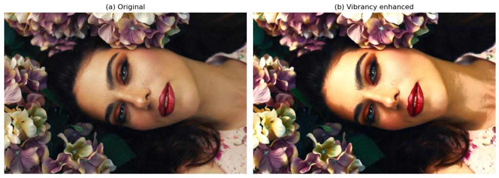
Figure 6. Compare the original photo (left) with vibrancy enhanced (right).
Enhance brightness
The Youtube tutorial achieved this by adding a "Levels" type "adjustment layer" on top of the dot-pattern layer, and changing the adjustment layer’s "blend mode" to screen.
Well this is truly mysterious. If you have some experiences with Photoshop, you may agree that blend modes are among the most difficult things to grasp. It’s just impossible for me to replicate the same effects of that "screen-mode-blended Levels adjustment layer". Oh I forgot to mention that the "transparency" level of the adjustment layer was also dropped to 50 % in the video.
Therefore, I will only attempt to implement something that will make the image "looks brighter", in the most general sense.
I found this post, Photoshop Blend Modes Explained, which gives a pretty in-depth explanation of the different blend modes. I took out the equation for the screen mode:
1 - (1 - A) * (1 - B)
where A is the layer on top, and B the one underneath, both have
been standardized to the range of [0, 1].
Seeing simple formula like this feels a bliss. So here is the Python function:
def screenBlend(image1, image2, alpha=1):
    '''Blend 2 layers using "screen" mode

    Args:
        image1 (ndarray): the layer on top.
        image2 (ndarray): the layer underneath. Both image1 and image2 are in
           range [0, 255].
    Returns:
        res (ndarray): blended image.

    Reference: https://photoblogstop.com/photoshop/photoshop-blend-modes-explained
    '''
    image1 = image1 / 255.
    image2 = image2 / 255.
    res =  1 - (1 - image1 * alpha) * (1 - image2)
    res = np.clip(res * 255, 0, 255)
    return res
Note that I’m not sure how to achieve the "transparency level" of
the blend mode, so my solution is the alpha keyword argument.
Below is the function call that works on the vibrancy-enhanced image:
# mimic a screen blend mode
filtered_vib_srn = screenBlend(filtered_vib, filtered_vib, 0.7)
Summary
In this post we mimic a dot pattern portrait effect originally achieved in Photoshop, using some simple Python code.
The below figure shows the entire process, from original photo in (a), to the application of the dot pattern in (b), the color vibrancy enhancement in (c), and brightness enhancement in (d). The color adjustment steps are a bit sketchy, but the overall effect is not too shabby. You might find this thing useful, for instance, for batch-processing some photos.
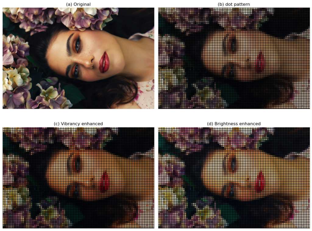
Figure 7. (a) Original photo. (b) Apply dot pattern stencils. (c) Apply vibrancy enhancement. (d) Apply brightness enhancement.
Lastly, below is the link to the complete script:
Recommend
About Joyk
Aggregate valuable and interesting links.
Joyk means Joy of geeK