SDP cones in BMIBNB

SDP cones in BMIBNB

Note: The support for nonlinear semidefinite programming is about to be significantly improved in an upcoming release. Forgot to post this article when the feature was added in 2020. Stay tuned!

YALMIP has an internal very general global solver BMIBNB. Since inception some 15 years ago, it has supported nonlinear semidefinite constraints (this is actually why it initially was developed as a quick experiement and 10 lines of code to test the internal infrastructure of YALMIP, hence the somewhat odd name) but this feature has essentially been useless as it required a nonlinear SDP solver for the upper bound and solution generation. Although PENSDP and PENBMI are such solvers (albeit limited in scope), they are not robust enough to be used in the branch & bound framework, and the development of these solvers appear to have stalled.

In release 20200930, the situation is improved with better support for the semidefinite cone in BMIBNB, and a completely different approach is used to achieve this. Instead of relying on external (non-existent) nonlinear SDP solvers, the machinery for the upper bound problem is based on a nonlinear cutting plane strategy using your standard favorite nonlinear solver. Will this work on any problem? Absolutely not. Will it work on most problems? No. A cutting plane strategy performs pretty badly already in the linear SDP case, but you might be lucky though, and this is work in progress.

Suitable background

To avoid repetition of general concepts, you are recommended to read the post on CUTSDP where cutting planes are used for the linear semidefinite cone in a different context. You are also adviced to read the general posts on global optimization and envelope generation to understand how a spatial branch & bound solver works.

The strategy

Having read the recommended articles, you know that BMIBNB needs three central components: A lower bound solver which solves a convex typically linear relaxation of the problem, an upper bound solver which tries to solve the original nonlinear problem starting from some suitably selected starting-point (typically some combination of the center of the currently investigated box and the solution to the lower bound problem), and a large collection of tricks to perform bound propagation to make it work in practice.

The lower bound problem does not pose any particular problem when we add a semidefinite cone to the model. After relaxing nonlinearities all we have to do is to solve a linear semidefinte program, which we have a plethora of solvers for. Hence, the only difference is that we swtich from a linear programming based lower bound (or more generally a quadratic or second-order cone programming solver) to a linear semidefinite programming solver. All bound propagation tricks applies also when there are semi-definite cones in model, and do not pose any complication either (on the contrary as a more general class of relaxations allows us to add more tricks).

The upper bound is the issue. While there are many solvers available for standard nonlinear programming, this is not the case for nonlinear programming involving semidefinite cones. In principle, if our nonlinear model has a semidefinite constraint G(x)⪰0, possibly nonlinear, we can view this as vTG(x)v≥0 ∀v. Hence, by simply adding an infinite number of scalar constraints, we can mimic the semidefinite constraint and solve the upper bound problem using a standard nonlinear solver. There is really nothing different concpetually to such a cutting plane approach compared to the linear case. Of course, this is not practical nor possible in reality.

Instead, we use the idea iteratively and build an approximation of the semidefinite cone as we work our way through the branching tree. Remember, it is not crucial that we actually manage to find a feasible solution in every node. It is of course good if we generate a feasible solution, but if we fail, it only means we have to open more nodes and try to find feasible solutions with associated upper bounds in those future nodes. Also remember that the upper bound problem is solved on a globally valid model. A semidefinite cut added to the upper bound model is valid in all nodes.

Hence, the obvious algorithm is

1. In the root node, create some initial approximation A of the semidefinite constraints G(x)⪰0 (e.g., add the constraint that the diagonal is non-negative)

2. In a node, solve the nonlinear program using the approximation A. If a solution is found, and G(x)⪰0 is satisfied, a valid upper bound has been computed. If G(x)⪰0 is violated, we do not have a feasible solution and thus no upper bound, but we can compute an eigenvector v associated to a negative eigenvalue and append the (possibly nonlinear) cut vTG(x)v≥0 to the approximation A.

3. Either repeat (2) several times in the node, or proceed with the branching process and use the new approximation in future nodes.

Everything else is exactly as before in the branch & bound algorithm.

Illustrating the steps manually

Consider a small example where we want to minimize x2+y2 over −3≤(x,y)≤3 and

G(x,y)=(y2−1x+yx+y1)⪰0.

The semidefinite constraint can also be written as y2−1≥0 and y2−1−(x+y)2≥0 by studying conditions for the matrix to be positive semidefinite (the first condition is redundant as it is implied by the second)

The feasible set is two disjoint regions top left and bottom right with borders outlined in red in the figure below.

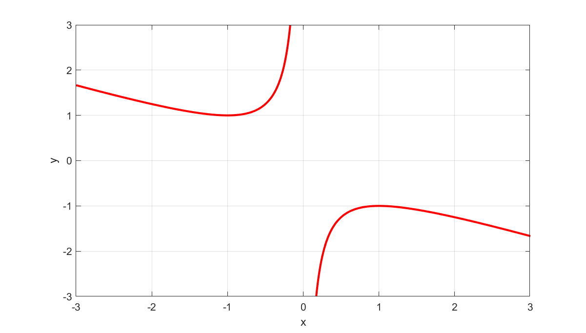
The figure can be generated with the following code

clf;
l=ezplot('y^2-1-(x+y)^2',[-3 3 -3 3]);
set(l,'color','red');set(l,'linewidth',2);
hold on
grid on

As an initial approximation of the feasible set, in addition to the box constrants, we have the nonconvex diagonal requirement y2−1≥0. This is the region above the top black line, and below the bottom black line in the following figure

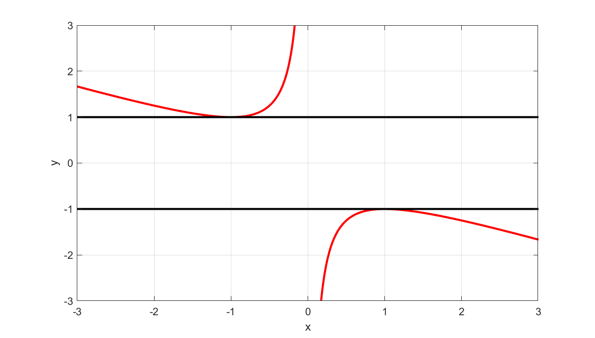
To generate these lines we run

l=ezplot('y^2-1-0*x',[-3 3 -3 3]);
set(l,'color','black');set(l,'linewidth',2);

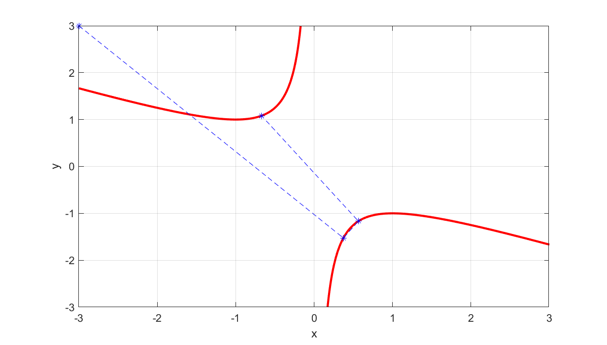
Now assume we use this initial model for upper bound generation. A nonlinear solver might find the solution x=0,y=1 marked with a black star in the figure below. Plugging in this solution into G(x,y) and computing eigenvalues shows that the matrix is indefinite (it is obviously not positive definite since the solution is outside the feasible region) meaning we failed to find a feasible solution to the original problem and thus generated no upper bound. By computing the associated eigenvector and forming the cut, we obtain a feasible region whose border is shown in blue. The feasible region to this cut is the area to the left of the blue curve. Note that it is tangent to the true feasible set at two points.Our nonlinear model is now the intersection of the two regions defined by the black lines, and the new region to the left of the blue line.

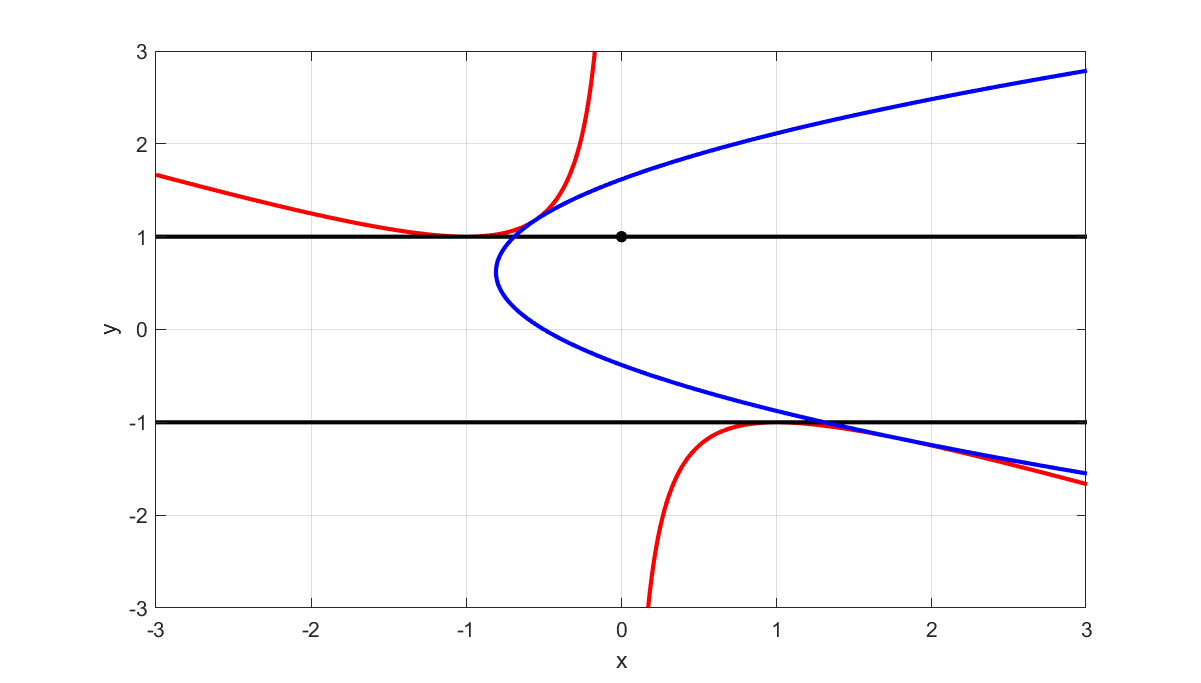
The computations are straightforward

l = plot(0,1,'ko');
set(l,'MarkerFaceColor','black')
sdpvar x y
G = [y^2-1 x+y;x+y 1]
assign([x;y],[0;1])
[V,D] = eig(value(G));
gi = V(:,1)'*G*V(:,1);
s = sdisplay(gi);
l = ezplot(s{1},[-3 3 -3 3]);
set(l,'color','blue');set(l,'linewidth',2);

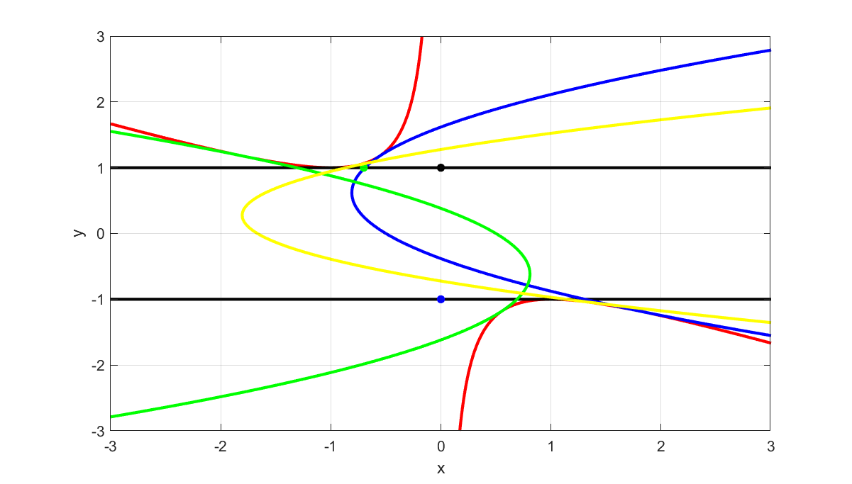
Once again, either in the same node or later on, the new model is used by the nonlinear solver, and this time we might obtain x=0,y=−1 marked with a blue star. We are still infeasible in the original model and analyzing eigenvalues and generating a new cut leads to the region to the right of the green curve. Iterating again using the intersection of the three constraints leads to, say, (-0.7,1) and a cut illustrated by the yellow line which we should be to the left of.

assign([x;y],[0;-1])
l = plot(0,-1,'bo');
set(l,'MarkerFaceColor','blue')
[V,D] = eig(value(G));
gi = V(:,1)'*G*V(:,1);
s = sdisplay(gi);
l = ezplot(s{1},[-3 3 -3 3]);
set(l,'color','green')
set(l,'linewidth',2);
l = plot(-.7,1,'go');
set(l,'Markersize',5)
set(l,'MarkerFaceColor','green')
assign([x;y],[-.7;1])
[V,D] = eig(value(G));
gi = V(:,1)'*G*V(:,1);
s = sdisplay(gi);
l = ezplot(s{1},[-3 3 -3 3]);
set(l,'color','yellow');
set(l,'linewidth',2);

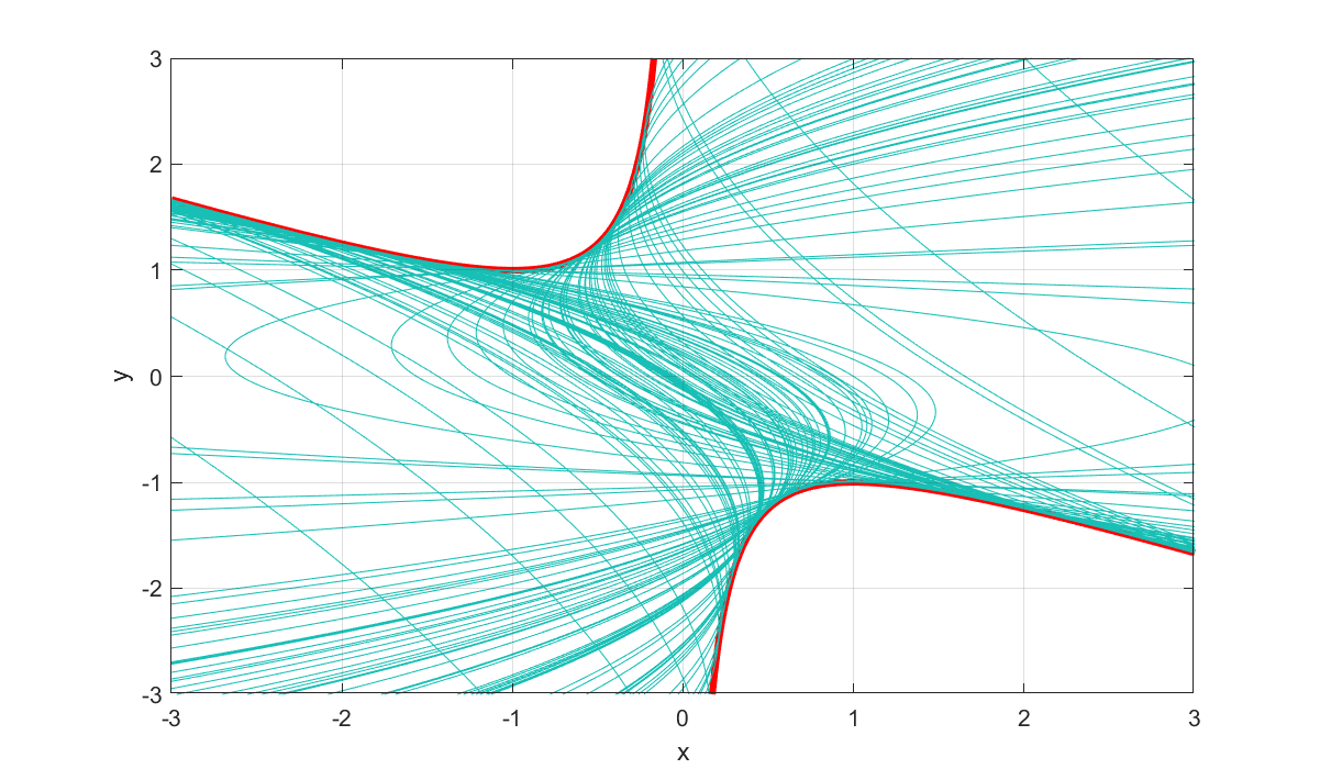
Just for fun, let us see what happens in the limit by generating cuts from a bunch of random points. Note that the choice of points is arbitrary. Here we draw it from the box, but we could just as well have drawn them on the unit circle, as the cut is scale invariant.

clf;
l=ezplot('y^2-1-(x+y)^2',[-3 3 -3 3]);
set(l,'color','red');set(l,'linewidth',3);
hold on
grid on
for i = 1:100
    assign([x;y],-3 + rand(2,1)*6);    
    [V,D] = eig(value(G));
    gi = V(:,1)'*G*V(:,1);
    s = sdisplay(gi);
    l = ezplot(s{1},[-3 3 -3 3]);
    drawnow
end

Running the solver

Let us test BMIBNB on the problem (we save some solver output for later analysis). From the log, we see that the algorithm found a feasible solution already in the first node (as we will see later, this is a trivial point in the top left corner). It then saw a bunch of SDP-infeasible solutions from which it generated cuts to add to the upper model, and after 5 iterations it found a new and better solution. More cuts were added, and in iteration 9 and 15 even better solutions were found, and with the solution found in node 15 the gap could be closed completely and thus a globally optimal solution was found. Note that the log tells us that the SDP-feasible solutions were not found by the upper-bound solver FMINCON, but were recovered using heuristics. The solutions generated by the upper bound solver are important though in generating relevant points to compute new cuts.

sdpvar x y
G = [y^2-1 x+y;x+y 1]
Model = [-3 <= [x y] <= 3, G >= 0];
sol = optimize(Model,x^2+y^2,sdpsettings('solver','bmibnb','savesolveroutput',1));
* Starting YALMIP global branch & bound.
* Upper solver     : fmincon
* Lower solver     : MOSEK
* LP solver        : GUROBI
* -Extracting bounds from model
* -Perfoming root-node bound propagation
* -Calling upper solver (no solution found)
* -Branch-variables : 2
* -More root-node bound-propagation
* -Performing LP-based bound-propagation 
* -And some more root-node bound-propagation
* Starting the b&b process
 Node       Upper       Gap(%)       Lower     Open   Time
    1 :   1.80000E+01   161.90    1.00000E+00    2     0s  Solution found by heuristics | Added 1 cut on SDP cone  
    2 :   1.80000E+01   161.90    1.00000E+00    3     0s  Added 1 cut on SDP cone  
    3 :   1.80000E+01   152.45    1.56312E+00    4     0s  Added 1 cut on SDP cone  
    4 :   1.80000E+01   152.45    1.56312E+00    5     0s  Added 1 cut on SDP cone  
    5 :   2.46872E+00    30.03    1.56312E+00    6     0s  Improved solution found by heuristics | Added 1 cut on SDP cone  
    6 :   2.46872E+00    30.03    1.56312E+00    5     0s  Added 1 cut on SDP cone | Pruned stack based on new upper bound  
    7 :   2.46872E+00    28.68    1.59858E+00    4     0s  Added 1 cut on SDP cone | Pruned stack based on new upper bound  
    8 :   2.46872E+00    28.68    1.59858E+00    5     0s  Added 1 cut on SDP cone  
    9 :   1.68243E+00     3.18    1.59858E+00    6     0s  Improved solution found by heuristics | Added 1 cut on SDP cone  
   10 :   1.68243E+00     3.18    1.59858E+00    3     0s  Poor bound in lower, killing node | Pruned stack based on new upper bound  
   11 :   1.68243E+00     2.60    1.61371E+00    4     0s  Added 1 cut on SDP cone  
   12 :   1.68243E+00     2.60    1.61371E+00    5     0s  Added 1 cut on SDP cone  
   13 :   1.68243E+00     2.60    1.61371E+00    6     0s  Added 1 cut on SDP cone  
   14 :   1.68243E+00     2.60    1.61371E+00    7     0s  Added 1 cut on SDP cone  
   15 :   1.61808E+00     0.00    1.61803E+00    0     0s  Poor bound in lower, killing node | Pruned stack based on new upper bound  
* Finished.  Cost: 1.6181 (lower bound: 1.618, relative gap 0%)
* Termination with all nodes pruned 
* Timing: 39% spent in upper solver (14 problems solved)
*         8% spent in lower solver (19 problems solved)
*         32% spent in LP-based domain reduction (76 problems solved)
*         3% spent in upper heuristics (73 candidates tried)

The figure below shows the progress of the upper bound solutions

clf;
l=ezplot('y^2-1-(x+y)^2',[-3 3 -3 3]);
set(l,'color','red');set(l,'linewidth',2);
hold on
grid on
plot(xhist(1,:),xhist(2,:),'b*--')

There’s more to the story

As explained above, nothing prevents us from iterating the cut-generating strategy in every node several times. This can be controlled by an option. If we want to perform, say, three rounds of solving the nonlinear program followed by adding violated SDP cuts, we run the code below. We see that several rounds are performed in every node, and the result is that more effort is spent in every node but a fewer number of nodes are needed. Note that it is not necessarily a good thing to add many new cuts in every node and strive for an SDP feasible solution everywhere. We might be wasting a lot of resources in creating a high-fidelity model in a region which is far from the globlly optimal solution anyway.

sdpvar x y
G = [y^2-1 x+y;x+y 1]
Model = [-3 <= [x y] <= 3, G >= 0];
sol = optimize(Model,x^2+y^2,sdpsettings('solver','bmibnb','bmibnb.uppersdprelax',3));
* Starting YALMIP global branch & bound.
* Upper solver     : fmincon
* Lower solver     : MOSEK
* LP solver        : GUROBI
* -Extracting bounds from model
* -Perfoming root-node bound propagation
* -Calling upper solver (no solution found)
* -Branch-variables : 2
* -More root-node bound-propagation
* -Performing LP-based bound-propagation 
* -And some more root-node bound-propagation
* Starting the b&b process
 Node       Upper       Gap(%)       Lower     Open   Time
    1 :   1.80000E+01   161.90    1.00000E+00    2     0s  Solution found by heuristics | Added 1 cut on SDP cone | Added 1 cut on SDP cone | Added 1 cut on SDP cone  
    2 :   1.80000E+01   161.90    1.00000E+00    3     0s  Added 1 cut on SDP cone | Added 1 cut on SDP cone | Added 1 cut on SDP cone  
    3 :   1.80000E+01   152.45    1.56312E+00    4     0s  Added 1 cut on SDP cone | Added 1 cut on SDP cone | Added 1 cut on SDP cone  
    4 :   1.80000E+01   152.45    1.56312E+00    5     0s  Added 1 cut on SDP cone | Added 1 cut on SDP cone | Added 1 cut on SDP cone  
    5 :   2.46872E+00    30.03    1.56312E+00    6     0s  Improved solution found by heuristics | Added 1 cut on SDP cone | Added 1 cut on SDP cone | Improved solution found by upper solver  
    6 :   2.46870E+00    30.03    1.56312E+00    5     0s  Added 1 cut on SDP cone | Added 1 cut on SDP cone | Improved solution found by upper solver | Pruned stack based on new upper bound  
    7 :   2.46870E+00    28.68    1.59858E+00    4     0s  Added 1 cut on SDP cone | Added 1 cut on SDP cone | Added 1 cut on SDP cone | Pruned stack based on new upper bound  
    8 :   1.61803E+00     0.75    1.59858E+00    5     0s  Added 1 cut on SDP cone | Improved solution found by upper solver  
* Finished.  Cost: 1.618 (lower bound: 1.5986, relative gap 0.74589%)
* Termination with relative gap satisfied 
* Timing: 69% spent in upper solver (9 problems solved)
*         5% spent in lower solver (12 problems solved)
*         14% spent in LP-based domain reduction (38 problems solved)
*         1% spent in upper heuristics (36 candidates tried)

This can be taken to the extreme. By setting the number of rounds to infinity, we force BMIBNB to continue adding SDP cuts until the solution either is SDP-feasible, or the nonlinear solver fails to find a solution to the approximation.

Another use of the framework is to use it in combintion with an external global solver. By using a global solver as the upper bound solver (!), and then setting the number of rounds to infinity, the solution computed will not only be SDP-feasible, but globally optimal! Since we know the computed solution is the globally optimal solution, we can terminate without bothering about the lower bound, and we can achive this by setting the lower bound target. Since our SDP cuts are quadratic, and the objective is quadratic, we can use Gurobi which supports global optimization for quadratic models. There is one tricky caveat here though: The numerical tolerances in BMIBNB vs Gurobi for judging feasibility can infer with each other. A solution which Gurobi thinks is good enough might still, according to BMIBNB, violate the cut we just added, and then we might keep adding the same cut in an infinite loop. To counteract this, we tighten the feasibility tolerance in Gurobi (and in pratice you would not want to set the iteration limit to infinity but something more sensible)

sdpvar x y
G = [y^2-1 x+y;x+y 1]
Model = [-3 <= [x y] <= 3, G >= 0];
ops = sdpsettings('solver','bmibnb','bmibnb.uppersdprelax',inf,'bmibnb.lowertarget',-inf);
ops = sdpsettings(ops,'bmibnb.uppersolver','gurobi','gurobi.FeasibilityTol',1e-8);
sol = optimize(Model,x^2+y^2,ops);
* Starting YALMIP global branch & bound.
* Upper solver     : GUROBI
* Lower solver     : MOSEK
* LP solver        : GUROBI
* -Extracting bounds from model
* -Perfoming root-node bound propagation
* -Calling upper solver (found a solution!)
* -Branch-variables : 2
* -More root-node bound-propagation
* -Performing LP-based bound-propagation 
* -And some more root-node bound-propagation
* -Terminating in root as solution found and lower target is -inf
* Timing: 79% spent in upper solver (1 problems solved)
*         7% spent in lower solver (4 problems solved)
*         0% spent in LP-based domain reduction (0 problems solved)
*         0% spent in upper heuristics (0 candidates tried)

Yet another application is to use the global framework as a trick to create a local nonlinear SDP solver. Just run it with any nonlinear solver until SDP-feasible, and then terminate by setting lower bound target to negative infinity. Note in the display below shows that in the root node, fmincon fails to even find a feasible solution to the SDP relaxed problem, and then no cuts can be generated. The SDP-feasible solution is actually found by heuristics for this particular example.

sdpvar x y
G = [y^2-1 x+y;x+y 1]
Model = [-3 <= [x y] <= 3, G >= 0];
ops = sdpsettings('solver','bmibnb','bmibnb.uppersdprelax',inf,'bmibnb.lowertarget',-inf);
ops = sdpsettings(ops,'bmibnb.uppersolver','fmincon');
sol = optimize(Model,x^2+y^2,ops);
* Starting YALMIP global branch & bound.
* Upper solver     : fmincon
* Lower solver     : MOSEK
* LP solver        : GUROBI
* -Extracting bounds from model
* -Perfoming root-node bound propagation
* -Calling upper solver (no solution found)
* -Branch-variables : 2
* -More root-node bound-propagation
* -Performing LP-based bound-propagation 
* -And some more root-node bound-propagation
* Starting the b&b process
 Node       Upper       Gap(%)       Lower     Open   Time
    1 :   1.80000E+01   161.90    1.00000E+00    2     0s  Solution found by heuristics  
* Finished.  Cost: 18 (lower bound: 1, relative gap 161.9048%)
* Termination with upper bound limit reached 
* Timing: 72% spent in upper solver (1 problems solved)
*         5% spent in lower solver (5 problems solved)
*         4% spent in LP-based domain reduction (4 problems solved)
*         2% spent in upper heuristics (4 candidates tried)