5 algorithms to train a neural network

5 algorithms to train a neural network

By Alberto Quesada, Artelnics.

The optimization algorithm (or optimizer) carries out the learning process in a neural network.

There are many different optimization algorithms. All of them are different in terms of memory requirements, processing speed, and numerical precision.

This post first formulates the learning problem for neural networks. Then, it describes some important optimization algorithms. Finally, it compares those algorithms' memory, speed, and precision.

Neural Designer includes many different optimization algorithms This allows you to always get the best models from your data. You can download a free trial here.

Learning problem

The learning problem is formulated as the minimization of a loss index, ff. It is a function that measures the performance of a neural network on a data set.

The loss index includes, in general, an error and a regularization terms. The error term evaluates how a neural network fits the data set. The regularization term prevents overfitting by controlling the model's' complexity.

The loss function depends on the adaptative parameters (biases and synaptic weights) in the neural network. We can group them into a single n-dimensional weight vector ww.

The next figure represents the loss function f(w)f(w).

As we can see, the minimum of the loss function occurs at the point w∗w∗. At any point AA, we can calculate the first and second derivatives of the loss function.

The gradient vector groups the first derivatives,

∇if(w)=∂f∂wi,∇if(w)=∂f∂wi,

for i=1,…,ni=1,…,n.

Similarly, the Hessian matrix gropus the second derivatives,

Hi,jf(w)=∂2f∂wi∂wj,Hi,jf(w)=∂2f∂wi∂wj,

for i,j=0,1,…i,j=0,1,….

The problem of minimizing continuous and differentiable functions of many variables is widely studied. We can directly apply many conventional approaches to this problem to training neural networks.

One-dimensional optimization

Although the loss function depends on many parameters, one-dimensional optimization methods are of great importance here. Indeed, they are very often used in the training process of a neural network.

Many training algorithms first compute a training direction dd and then a training rate ηη that minimizes the loss in that direction, f(η)f(η). The next figure illustrates this one-dimensional function.

The points η1η1 and η2η2 define an interval that contains the minimum of ff, η∗η∗.

In this regard, one-dimensional optimization methods search for the minimum of one-dimensional functions. Some of the most used are golden section and the Brent's method. Both reduce the minimum bracket until the distance between the two outer points is less than a defined tolerance.

Multidimensional optimization

The learning problem for neural networks is formulated as searching of a parameter vector w∗w∗ at which the loss function ff takes a minimum value. The necessary condition states that if the neural network is at a minimum of the loss function, then the gradient is the zero vector.

The loss function is, in general, a non-linear function of the parameters. Consequently, it is impossible to find closed training algorithms for the minima. Instead, we consider a search through the parameter space consisting of a succession of steps. At each step, the loss will decrease by adjusting the neural network parameters.

In this way, to train a neural network, we start with some parameter vector (often chosen at random). Then, we generate a sequence of parameters, so that the loss function is reduced at each iteration of the algorithm. The change of loss between two steps is called the loss decrement. The training algorithm stops when a specified condition, or stopping criterion, is satisfied.

1. Gradient descent

Gradient descent is the most straightforward training algorithm. It requires information from the gradient vector, and hence it is a first-order method.

Let denote f(w(i))=f(i)f(w(i))=f(i) and ∇f(w(i))=g(i)∇f(w(i))=g(i). The method begins at a point w(0)w(0) and, until a stopping criterion is satisfied, moves from w(i)w(i) to w(i+1)w(i+1) in the training direction d(i)=−g(i)d(i)=−g(i). Therefore, the gradient descent method iterates in the following way:

w(i+1)=w(i)−g(i)η(i),w(i+1)=w(i)−g(i)η(i),

for i=0,1,…i=0,1,….

The parameter ηη is the training rate. This value can either be set to a fixed value or found by one-dimensional optimization along the training direction at each step. An optimal value for the training rate obtained by line minimization at each successive step is generally preferable. However, there are still many software tools that only use a fixed value for the training rate.

The next picture is an activity diagram of the training process with gradient descent. As we can see, the algorithm improves the parameters in two steps: First, it computes the gradient descent training direction. Second, it finds a suitable training rate.

The gradient descent training algorithm has the severe drawback of requiring many iterations for functions that have long, narrow valley structures. Indeed, the downhill gradient is the direction in which the loss function decreases the most rapidly, but this does not necessarily produce the fastest convergence. The following picture illustrates this issue.

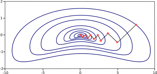
Gradient descent is the recommended algorithm when we have massive neural networks, with many thousand parameters. The reason is that this method only stores the gradient vector (size nn), and it does not store the Hessian matrix (size n2n2).

2. Newton's method

Newton's method is a second-order algorithm because it uses the Hessian matrix. This method's objective is to find better training directions by using the second derivatives of the loss function.

Let denote f(w(i))=f(i)f(w(i))=f(i), ∇f(w(i))=g(i)∇f(w(i))=g(i) and Hf(w(i))=H(i)Hf(w(i))=H(i). Consider the quadratic approximation of ff at w(0)w(0) using the Taylor's series expansion

f=f(0)+g(0)⋅(w−w(0))+0.5⋅(w−w(0))2⋅H(0)f=f(0)+g(0)⋅(w−w(0))+0.5⋅(w−w(0))2⋅H(0)

H(0)H(0) is the Hessian matrix of ff evaluated at the point w(0)w(0). By setting gg equal to 00 for the minimum of f(w)f(w), we obtain the next equation

g=g(0)+H(0)⋅(w−w(0))=0g=g(0)+H(0)⋅(w−w(0))=0

Therefore, starting from a parameter vector w(0)w(0), Newton's method iterates as follows

w(i+1)=w(i)−H(i)−1⋅g(i)w(i+1)=w(i)−H(i)−1⋅g(i)

for i=0,1,…i=0,1,….

The vector H(i)−1⋅g(i)H(i)−1⋅g(i) is known as Newton's step. Note that this parameter change may move towards a maximum rather than a minimum. This occurs if the Hessian matrix is not positive definite. Thus, Newton's method does not guarantee to reduce the loss index at each iteration. To prevent that, Newton's method equation is usually modified as:

w(i+1)=w(i)−(H(i)−1⋅g(i))ηw(i+1)=w(i)−(H(i)−1⋅g(i))η

for i=0,1,…i=0,1,….

The training rate, ηη, can either be set to a fixed value or found by line minimization. The vector d(i)=H(i)−1⋅g(i)d(i)=H(i)−1⋅g(i) is now called Newton's training direction.

The following figure depicts the state diagram for the training process with Newton's method. The parameters are improved by first obtaining Newton's training direction and then a suitable training rate.

The picture below illustrates the performance of this method. As we can see, Newton's method requires fewer steps than gradient descent to find the minimum value of the loss function.

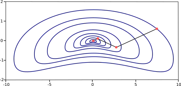
However, Newton's method has the difficulty that the exact evaluation of the Hessian and its inverse are pretty expensive in computational terms.

3. Conjugate gradient

The conjugate gradient method can be regarded as something intermediate between gradient descent and Newton's method. It is motivated to accelerate the typically slow convergence associated with gradient descent. This method also avoids the information requirements associated with the Hessian matrix's storage, evaluation, and inversion, as Newton's method requires.

In the conjugate gradient training algorithm, the search is performed along with conjugate directions. They generally produce faster convergence than gradient descent directions. These training directions are conjugated concerning the Hessian matrix.

Let denote d the training direction vector. Then, starting with an initial parameter vector w(0)w(0) and an initial training direction vector d(0)=−g(0)d(0)=−g(0), the conjugate gradient method constructs a sequence of training directions as:

d(i+1)=g(i+1)+d(i)⋅γ(i),d(i+1)=g(i+1)+d(i)⋅γ(i),

for i=0,1,…i=0,1,….

Here γγ is called the conjugate parameter, and there are different ways to calculate it. Two of the most used are due to Fletcher and Reeves and Polak and Ribiere. For all conjugate gradient algorithms, the training direction is periodically reset to the negative of the gradient.

The parameters are then improved according to the following expression.

w(i+1)=w(i)+d(i)⋅η(i)w(i+1)=w(i)+d(i)⋅η(i)

for i=0,1,…i=0,1,….

The training rate, ηη, is usually found by line minimization.

The picture below depicts an activity diagram for the training process with the conjugate gradient. Here improvement of the parameters is done in two steps. First, the algorithm computes the conjugate gradient training direction. Second, it finds a suitable training rate in that direction.

This method has proved to be more effective than gradient descent in training neural networks. Since it does not require the Hessian matrix, the conjugate gradient also performs well with vast neural networks.

4. Quasi-Newton method

The application of Newton's method is computationally expensive. Indeed, it requires many operations to evaluate the Hessian matrix and compute its inverse. Alternative approaches, known as quasi-Newton, are developed to solve that drawback. These methods do not calculate the Hessian directly and then evaluate its inverse. Instead, they build up an approximation to the inverse Hessian. This approximation is computed using only information on the first derivatives of the loss function.

The Hessian matrix is composed of the second partial derivatives of the loss function. Thus, the main idea behind the quasi-Newton method is approximating the inverse Hessian by another matrix GG, using only the first partial derivatives of the loss function. Then, the quasi-Newton formula is expressed as

w(i+1)=w(i)−(G(i)⋅g(i))⋅η(i)w(i+1)=w(i)−(G(i)⋅g(i))⋅η(i)

for i=0,1,…i=0,1,….

The training rate ηη can either be set to a fixed value or found by line minimization. The inverse Hessian approximation GG has different flavors. Two of the most used ones are the Davidon–Fletcher–Powell (DFP) and the Broyden–Fletcher–Goldfarb–Shanno (BFGS) formulas.

The activity diagram of the quasi-Newton training process is illustrated below. Improvement of the parameters is performed in two steps. First, the algorithms obtains the quasi-Newton training direction. Second, it finds a satisfactory training rate.

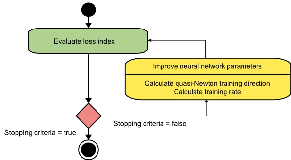
This is the default method to use in most cases: It is faster than gradient descent and conjugate gradient, and the exact Hessian does not need to be computed and inverted.

5. Levenberg-Marquardt algorithm

The Levenberg-Marquardt algorithm is designed to work specifically with loss functions which take the form of a sum of squared errors. It works without computing the exact Hessian matrix. Instead, it works with the gradient vector and the Jacobian matrix.

Consider a loss function which takes the form of a sum of squared errors,

f=m∑i=1e2if=∑i=1mei2

Here mm is the number of training samples.

We can define the Jacobian matrix of the loss function as that containing the derivatives of the errors concerning the parameters,

Ji,j=∂ei∂wj,Ji,j=∂ei∂wj,

for i=1,…,mi=1,…,m and j=1,…,nj=1,…,n.

Where mm is the number of samples in the data set, and nn is the number of parameters in the neural network. Note that the size of the Jacobian matrix is m⋅nm⋅n.

We can compute the gradient vector of the loss function as

∇f=2JT⋅e∇f=2JT⋅e

Here ee is the vector of all error terms.

Finally, we can approximate the Hessian matrix with the following expression.

Hf≈2JT⋅J+λIHf≈2JT⋅J+λI

Where λλ is a damping factor that ensures the positiveness of the Hessian and II is the identity matrix.

The next expression defines the parameters improvement process with the Levenberg-Marquardt algorithm

w(i+1)=w(i)−(J(i)T⋅J(i)+λ(i)I)−1⋅(2J(i)T⋅e(i)),w(i+1)=w(i)−(J(i)T⋅J(i)+λ(i)I)−1⋅(2J(i)T⋅e(i)),

for i=0,1,…i=0,1,….

When the damping parameter λλ is zero, this is just Newton's method, using the approximate Hessian matrix. On the other hand, when λλ is large, this becomes gradient descent with a small training rate.

The parameter λλ is initialized to be large so that the first updates are small steps in the gradient descent direction. If any iteration results in a fail, then λλ is increased by some factor. Otherwise, as the loss decreases, λλ is reduced, so the Levenberg-Marquardt algorithm approaches the Newton method. This process typically accelerates the convergence to the minimum.

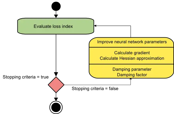
The picture below represents a state diagram for the training process of a neural network with the Levenberg-Marquardt algorithm. The first step is to calculate the loss, the gradient, and the Hessian approximation. Then the damping parameter is adjusted to reduce the loss at each iteration.

As we have seen, the Levenberg-Marquardt algorithm is a method tailored for functions of the type sum-of-squared-error. That makes it to be very fast when training neural networks measured on that kind of errors.

However, this algorithm has some drawbacks. First, it cannot minimize functions such as the root mean squared error or the cross-entropy error. Also, the Jacobian matrix becomes enormous for big data sets and neural networks, requiring much memory. Therefore, the Levenberg-Marquardt algorithm is not recommended when we have big data sets or neural networks.

Performance comparison

The following chart depicts the computational speed and the memory requirements of the training algorithms discussed in this post.

As we can see, the slowest training algorithm is usually gradient descent, but it is the one requiring less memory.

On the contrary, the fastest one might be the Levenberg-Marquardt algorithm, but it usually requires much memory.

A good compromise might be the quasi-Newton method.

Conclusions

To conclude, if our neural network has many thousands of parameters, we can use gradient descent or conjugate gradient, to save memory.

If we have many neural networks to train with just a few thousand samples and a few hundred parameters, the best choice might be the Levenberg-Marquardt algorithm.

In the rest of situations, the quasi-Newton method will work well.

Neural Designer implements all that optimization algorithms. You can download the free trial to see how they work in practice.

Do you need help? Contact us | FAQ | Privacy | © 2022, Artificial Intelligence Techniques, Ltd.