Binary Trees are optimal… except when they’re not. | Harder, Better, Faster, Str...

Binary Trees are optimal… except when they’re not.

The best case depth for a search tree is , if is the arity (or branching) of the tree. Intuitively, we know that if we increase , the depth goes down, but is that all there is to it? And if not, how do we chose the optimal branching ?

While it’s true that an optimal search tree will have depth , we can’t just increase indefinitely, because we also increase the number of comparisons we must do in each node. A -ary tree will have (in the worst case) keys, and for each, we must do comparisons for lower-than and equal (the right-most child will be searched without comparison, it will be the “else” of all the comparisons). We must first understand how these comparisons affect average search time.

If we use a naïve comparison scheme, each keys ask for two (potentially expensive) comparisons. One to test if the sought value, is smaller than a key ; one to test if they’re equal. If neither tests is true, we move on to the next key. If none of the tests are true, it is an “else” case and we go down the rightmost branch. That scheme does way more work than necessary and would ask for comparison per node (because there are keys per node).

The main problem with this straightforward approach is that comparisons can be very expensive. While comparing two integral types (int and the like) is often thought of as “free”, comparing string is expensive. So you clearly do not want to test two strings twice, once for < and once for =. The much better approach is to use a three-way comparison, also known as the “spaceship operator”.

The spaceship operator, <=> is C++20’s version of C’s old timey qsort comparison function (it is in fact much better because it also automagically provides all comparison operators). Basically, a<=>b can return <0 if a<b, 0 if they’re equal, and >0 if a>b. We can therefore store the result of the expensive comparison, then do inexpensive comparisons for the result. That reduces the number of expensive comparisons to per node.

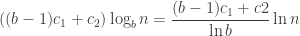
The search complexity, counting the number of comparisons in the worst case for the best-case tree is

,

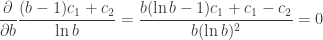
a strictly increasing function in (as we can treat as a constant, since we’re not optimizing for ):

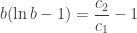
We therefore conclude that is the optimal solution.

Except when it isn’t

We have neglected, or rather abstracted, something important: the cost of accessing the node. In main memory, it’s very convenient to suppose that reading a node is free, that is, incurs no cost. That’s of course false, because even reading from cache incurs a delay; fortunately very small. It is even more false if we read the node from disk (yes, even NVMe). A classical spinning rust disk reading a block will cause a few millisecond delay, that may be really, really expensive relative to the comparison of two keys (once they’re) in memory.

The new cost function to optimize will be

,

with the comparison cost, and , the cost of accessing the node. We can set to 1 and make relative to . Let’s say something like . Now, luckily for us, this function is convex in , so we can solve for the optimal given and . To do so, we take the derivative and find where it is zero, that is, solve

for . Since the denominator is strictly increasing in , we must solve for a zero numerator. However, there’s a slight complication:

isn’t algebraic. We must use a numerical solution to the Lambert W Function. It gives us, with ,

.

The following graph shows the function’s surface with and , one axes being , block size and the other being , the number of items in the tree. The green plane shows the optimal found with the Lambert W function.

To conclude, binary trees are optimal when we ignore the cost of accessing a node, but they aren’t when it becomes costly to access a node. When we access the nodes on disk, with a high cost, it becomes interesting to bundles many keys in a node, and we gave the optimal solution. However, the problem is often solved quite more directly. We just fit as many keys as possible in an I/O block. Disks operates on small blocks of (typically) 512 bytes, but file systems operate in somewhat larger, but fixed-sized blocks, something like 4 or 8k. A good strategy is therefore to fit as many keys as possible in that block, since even if the number of comparisons is large, it will still be faster than bringing that block into main memory.

This entry was posted on Tuesday, July 20th, 2021 at 2:52 am and is filed under Uncategorized. You can follow any responses to this entry through the RSS 2.0 feed. You can leave a response, or trackback from your own site.

Post navigation