Representing line intersections as a system of linear equations

(Note: this article was originally written in and transcribed to WordPress, so forgive the equation alignment. Get the original).

In a previous post, I outlined an analytical solution for intersecting lines and
ellipses. In this post I’m doing much the same thing but rather with lines on lines. I’ll point out why the normal slope-intercept form for a line is a poor representation, and what we can do about that.

In computer graphics, or just geometry in general, you often find yourself in a scenario where you want to know if and how two or more objects intersect. For example, in the latest shooting game you’re playing perhaps a bullet is represented as a sphere and a target is represented as a disc. You want to know if the bullet you’ve fired has struck the target, and if so, was it a bulls-eye?

Where did the line hit the target?

In this post, I’ll step you through one way we can accomplish discovering intersection points between two lines, being sure to carefully walk through each step of the calculation so that you don’t get lost.

Slope-Intercept Form

We’re going to fly in the face of many approaches to line-line intersection here and try to ultimately wind up with a system of linear equations to solve. This is different from the “usual” way of finding intersections by crafting an equation to represent each geometric body, and then somehow setting those equations equal to each other. For example, if we used the familiar slope-intercept form to represent a line, we’d end up representing the lines as

(1)
(2)

Then afterwards we could solve for by assigning the equations to each other:

And with some algebraic fiddling, we could get , and the take that and insert it into either line equation in above to get .

But here are some questions to think about.

A problem

Slope-intercept form assumes two things:

1. Every line has a slope
2. Every line has a y-intercept

This is all well and good for most lines. Even horizontal lines have a slope of 0, and a y-intercept somewhere. Our problem is with perfectly vertical lines:

A vertical line segment (green) crosses a horizontal line (blue)

What is the slope of a vertical line, since the “run” part of rise-over-run, is zero? Vertical lines don’t touch the y-axis either unless they’re collinear with it, and even then there wouldn’t be just a single y-intercept.

Vertical lines are better represented as a function of . Like the part isn’t even here, it just doesn’t exist! That’s because there are infinite values of for our given .

One solution

Vertical lines are the bane of slope-intercept form’s existence. If both lines were vertical, we could test for that and then not bother with testing for intersection, but what if just one of them were vertical? How would we check for the intersection point then?

Well, let’s examine an alternative representation of a line. Those of you who have ever taken a linear algebra course should be familiar with it:

(3)

Where , , and are known constant values, and we’re solving for and .

Okay, what the heck is that? In the next section I’ll explain exactly how this solves our vertical line problem, but first I need to demonstrate to you how we can even get a line into that format.

Two-point form: an alternative representation for a line

“What? We don’t always use slope-intercept form??? All my teachers have lied to me!” In fact, there are many ways we can represent a line, and like any tool there’s a time and a place for each of them.

The representation we’re interested in here is called Two-point form. And we can derive it if we already have two points on the line (which is common if you have a bunch of line segments in the plane, like sketch strokes).

Given:
We have two points on the line,

we can represent a line in the following form, parameterized on and :

(4)

Still doesn’t seem to help us, does it? We’ve gotten rid of the intercept, but we still have a slope, which becomes a big problem when . So let’s fix that but multiplying both sides of the equation by :

(5)

(This is called Symmetric form) Let’s manipulate Equation 5 so that and (no subscripts) appear only once. Start by multiplying everything through:

We notice that the terms can cancel out:

Now we rearrange the left side in terms of :

And the right side in terms of :

Subtract the term from both sides:

and add the term:

Let’s move the equals sign to the other side:

And move the and to the other side of the parentheses:

Notice now how similar this equation is to Equation 3.

We can define:

Distributing the negative through for :

(6)

To be left with the same equation (restated here):

Line-line intersection via solving a system of linear equations

Now that we can represent a single line as a linear equation in two variables, and , we can represent the intersection of two lines as a system of linear equations in two variables:

Where we compute and by using the two-point form mathematics from the previous section. With two equations and two unknowns, we can compute and .

In the next part I will slowly walk through how we will solve this system using basic techniques from linear algebra
(Warning! Lots of math incoming!).

The idea behind solving a system of equations like this is to get it into something called row-echelon form, which is a fancy way of saying “I want the coefficient on in the top equation to be , and the coefficient of  in the bottom equation to be , with other coefficients of and to be zero”:

Let’s begin with getting the coefficient on in the top row to be . First divide through the top equation by :

Simplifying:

Notice that at this point, we’ve succeeded in getting a coefficient of on in the top equation.

The next thing we do is notice that, since we have a bare in the top equation, we could multiply it by and then subtract it from the in the bottom equation to get the bottom one’s coefficient on to be zero. However, we cannot do this solely on . Instead, we’re restricted to what are called Elementary Row Operations that limit what we can do while preserving the correctness of the equations. So what we have to do is multiply the entire top row by , and then subtract the top row from the bottom row, which looks like this:

Which gives us a coefficient on in the second row!

Let’s simplify the and terms in the second row to have a common denominator:

The next step is to get a coefficient of on the term in the second row by dividing through the row by , which results in us replacing the coefficient on with a , and then multiplying the third term by the flipped fraction (remember that when we divide two fractions, we flip the second one and then multiply):

We can cancel the terms in the multiplication, and the resulting equation becomes:

At this point, we’ve solved for . That is,

We could substitute for in the top row to solve for , but a more linear-algebra-ish way would be to perform another elementary row operation — multiply the bottom row by , and then subtract it from the top row. Here’s what that looks like:

Now we’ve achieved a coefficient of on the term in the top row!

We’ve essentially solved for at this point, but the term on the other side of the is a little ugly, and we can simplify it. Let’s start by making the two parts of the term have the same denominator, which means we need to multiply  by (which is really just multiplying by 1!):

Distributing the term in the numerator, and combining the terms because they have the same denominator:

When we distribute the in the numerator, the term becomes positive:

Which leaves us with both and $+a_2b_1c_1$ in the numerator, which cancel:

We can factor out in the numerator:

Finally, the terms in the numerator and denominator cancel, leaving us with:

Now we’re ready to say we’ve solved the linear system for and , leaving us with

(7)

Substituting the values from Equation 6 into Equation 7 yields:

(8)

This formulation is identical to the one you’ll find on Wikipedia (although they’ve arranged the denominators slightly differently, but still mathematically equivalent).

A caveat

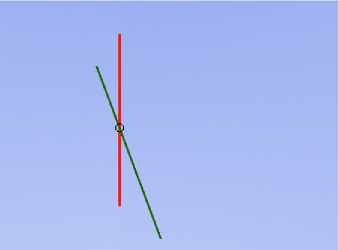
Ironically, despite all that extra math, we’ll still have problems with vertical lines, but only when those lines are parallel, which means there are either infinitely many solutions (lines are collinear) or zero solutions (lines are parallel but not collinear, like in the figure below).

Two vertical lines are problematic only because they’re parallel

Checking for parallel lines is fortunately pretty simple.

Checking for parallel lines

Let’s say we have two line segments floating around the Cartesian plane:

Two line segments in the x-y plane

To check for whether these are parallel, first imagine translating the lines so that they both have an endpoint at :

We’ve moved the lines so they start at the origin

There will be some angle between the two lines:

There is some angle, marked as between our lines

If this angle is , or radians (°) then will be .

Given that we are representing our lines using two points, we can use those points to create vectors, which are like our lines from the origin that have a length and a magnitude.

To create a vector given points and , we just subtract one from the other (for our purposes here it doesn’t matter the order!):

(9)

We draw them with little arrows to indicate a direction:

Our lines are now vectors

After we’ve created vectors for both our lines, we can take advantage of a mathematical relationship between them called the cross product to find whether they’re parallel or not. For two vectors  and , their cross product is defined as

(10)

Where and are the magnitudes of the vectors, which can be thought of as a vector’s “length”. For some vector , it’s defined as

(11)

However, for the sake of testing for parallel lines, what we’re really interested in is the term in the cross product, where is the smallest angle between the vectors (the vectors are simultaneously separated by and radians).

Assuming our vectors don’t have magnitudes of zero, when the cross product between them is zero (or really really close to zero) we consider the lines to be parallel because the angle between them must be zero. This tells us that the lines either never collide, or they’re infinitely colliding because they’re the same line (collinear). I leave checking for collinearity as an exercise to you.

A shortcut

One might say we solved our system of linear equations the long way. In fact, since we had exactly two equations and exactly two unknowns, we could have leveraged a mathematical technique known as Cramer’s rule. The method is actually not so hard to apply, but perhaps its correctness is a little more difficult to understand.

Conclusions

Checking for line-line intersections is a harder problem than it appears to be on the surface, but once we give it a little thought it all boils down to algebra.

One application for line-line intersection testing is in computer graphics. Testing for intersections is one of the foundational subroutines for computing Binary Space Partitioning (BSP) Trees, which are a way to efficiently represent a graphical scene, or even an individual object within a scene. BSP Trees are perhaps most famously known for their use by John Carmack in the Doom games.

In closing, we can consider a line in 2D to actually be a hyperplane that partitions the plane into areas “on one side or the other” the line. Therefore, there are analogs in 3D space where we use a 3D hyperplane (what we typically think of as a plane) to partition the space again into areas “on one side or the other” of the plane.

The original Doom used BSP trees for efficient scene representation