Representing plane intersections as a system of linear equations

Representing plane intersections as a system of linear equations – Andy G's BlogSkip to content Skip to menu

When you are watching a digitally-rendered battle onscreen in the latest blockbuster movie, you don’t always think about the “camera” moving about that scene. In the real-world, cameras have a field of view that dictates how much of the world about them they can see. Virtual cameras have a similar concept (called the viewing frustum) whereby they can only show so much of the digital scene. Everything else gets chopped off, so to speak. Because rendering a digital scene is a laborious task, computer scientists are very interested in making it go faster. Understandably, they only want to spend time drawing pixels that you’ll see in the final picture and forget about everything else (outside the field of view, or occluded (hidden) behind something else).

Our friends in the digital graphics world make heavy use of planes everyday, and being able to test for plane-plane intersection is extremely important.

In this post, I’ll try to break down what a plane is in understandable terms, how we can create one given a triangle, and how we would go about testing for the intersection between two of them.

(This article was originally written in and transcribed here. To get a hard copy that you can also cite, grab the pdf here)

What is a plane, anyway?

Say you’re given a triangle in 3D space. It consists of three points, , , and that each have , , and components:

For simplicity’s sake, we’ll assume that, moving “counter-clockwise”, the triangle’s points go in the order , , and then (and then back to ).

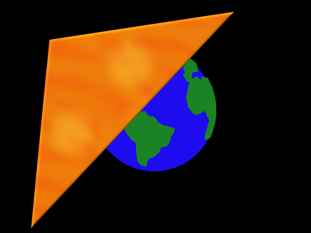
A triangle is distinctly “flat”. It’s like a perfectly constructed Dorito. Also, no matter which way you turn it and rotate it, there’s always a definite front and back. That is, if you extended the corners of your Dorito off towards infinity, then you could completely bisect the room, your state, the planet, the universe!

And feed a lot of hungry people, too

This ability to split a space in two is a salient feature of a plane, and we can construct one with the triangle we’ve just defined. In the next few sections we’ll go more into depth in exactly how to do that.

Normal vector

In the previous section I said that our gargantuan flat Dorito had two distinct sides, front and back. That means you could draw a straight line from the “back” that eventually comes out the “front”. Imagine that our Dorito is so large that it is its own planet orbiting the Sun. You could hop in a space ship, fly up to that Dorito, take one small step for man, and then plant your flag on top. In geometric terms, your flag pole would be the normal vector to the plane’s (Dorito’s) surface.

Our Dorito planet with a normal vector pointing “up” out of it

A normal vector  to a plane is a line that is perfectly perpendicular to any other line drawn entirely within the plane. We call it a vector because it has a direction associated with it. That is, the flag you planted on the Dorito planet points “up”, but you could just have easily landed on the other side and planted the flag pointing “down”, and it would still be perfectly valid; all we need is just to choose one.

Our normal vector will also have , , and components, but we’ll label them , , and to distinguish them from the points in the triangle:

Vector equation of a plane

At this point we have a triangle, but we only know about what a normal vector is. How do we compute the normal vector given a triangle’s points?

Our normal vector is perpendicular to any line we draw in the plane. In computer graphics terms, we say the normal vector is “orthogonal” to our plane. An nice example of orthogonality is that the Y-axis is perpendicular to the X-axis (and the Z-axis is perpendicular to both!).

In geometry, we know how to obtain a perpendicular vector (a normal vector) so long as we have 2 non-parallel vectors in the plane. But first we need to get those two vectors in the plane. So how do we do that?

Obtaining non-parallel vectors in a plane given a triangle

Remember from before that we defined our plane originally using three points, , , and . We can use these points to compute our vectors.

Think about it this way. The center of the earth is position , and you’re standing at some random point . Your friend Andy is standing at position . Vectors imply a direction, so how do you get a direction from you to your friend? Subtraction! You can compute your friend’s offset from yourself by subtracting your own position from Andy’s: . The resulting offset is a direction out from the center of the earth in the same direction as the direction from you to your friend.

If your other friend Bernhard is standing at position , you’d do the exact same thing to get a vector representing the direction from you to him. So long as all three of you are not standing in a line, you now have two non-parallel vectors. Fortunately, our original points , , and define a triangle, and none of the sides of that triangle are parallel, so we’re good.

In our example, you are standing at , Andy is at , and Bernhard is at . We can compute two non-parallel vectors, as

Computing a normal vector to a plane given two vectors in the plane

In geometry there is this fancy thing called a cross product that enables us to compute an orthogonal (perpendicular) vector so long as we are given two input vectors. What does this mean? Well, there are a couple different interpretations, and I’ll work up to them after first discussing something called a dot product.

The cross product is a special kind of multiplication. The multiplication you were taught in grade school resulted in numbers many times larger than they were before. For example, , which is quite bit larger than either or . The “problem” here is that doesn’t have any sense of direction to it!

Our grade school multiplication has a ready analog in the world of vectors (things that have direction) called the dot product: we start by  multiplying the components! Afterwards we add them all together to get a single value. The dot product can be thought of as “multiplication in the same direction” because we multiply the components together, the components together, as well as the components.

An alternate interpretation of the dot product is that it’s a measure of just “how much” in the same direction your two vectors are:

Where and are the magnitudes of the vectors:

and is the angle between them.

Two vectors with angle Θ between them

When is 0, the vectors are in the same direction (parallel), meaning the cosine is (it’s largest value) and therefore the result is the largest possible dot product between the two vectors. (Data miners love to use this and call it “cosine similarity”). But if the vectors were orthogonal (perpendicular), the dot product would be zero.

The cross product is similar to the dot product except it’s more of a measure of how different two vectors are. The data miners might choose the following representation of a cross product:

When the term is 0, the vectors are in the same direction (parallel), which maximizes the dot product, but the cross product is zero! And when is 90 degrees ( radians), the vectors are perpendicular and the cross product is maximized! (The dot product, sadly, becomes 0).

There exists another way to compute a cross product where the result is not a single number, but rather a vector that is orthogonal to both the input vectors:

 (1)

It’s not the most intuitive computation. Personally, I enjoyed the “xyzxyz” explanation at
Better Explained.

All we need to know is that the result of this equation is a shiny new orthogonal vector.

Putting it together

We now have two vectors in our plane, and , which we computed using our triangle’s points , , and . We also know how to take two vectors and compute an orthogonal vector. Our normal vector is exactly that; an orthogonal vector to our plane, so when we apply the cross product to and , we obtain our normal vector :

Which gives us

Now that we have a normal vector, we can define our plane intuitively. We know that our normal vector is perpendicular to all vectors in the plane, and as we saw before, the dot product of any two vectors is zero if the vectors are orthogonal. We can therefore say that, given our point on the plane, and any other point on the plane, the dot product between and (subtracting two points results in a vector) is :

(2)

Which is our generic representation of a plane. This is a nice way to think about a plane, but alone it doesn’t help us find the intersection between two planes. Ultimately what we want is a system of linear equations like the title talked about.

Representing a plane as a linear equation

Given our plane equation

Let’s expand the terms.

After performing the dot product:

Distributing , , and :

We know what the values of and are (they’re constants) because they were given to us in the plane’s definition, so let’s move them to the other side of the sign in order to have only variables on one side and only constants on the other.

and since is constant, it will be easier to relabel it as instead of writing it out every time. That is,

Which results in a linear equation that looks like this:

If we have two planes, then we’ll distinguish between their definitions via subscripts on our constant:

     (3)

Finally we have a system of linear equations. Great! We have ways to solve those! However, this particular one presents a little problem. (A tiny one that we’ll make go away)

A problem

In linear algebra, we are often provided with a number of equations and an equal number of unknowns (variables) we must solve for. However, in our system, we appear to have more variables than equations!

Let’s take another look.

We have three variables to solve for — , , , and yet only two equations. This is called an Under-determined system meaning there are infinite solutions (assuming the planes intersect at all). Infinite? You see, when a line intersects a line, they intersect at a single point, but when a plane intersects another plane, that intersection is a line, which has infinitely many points. We would need three planes to intersect before we could find a single point of intersection.

Solving an under-determined system

There are more math-intensive approaches to solving under-determined systems that involve computing something called a pseudo-inverse, but for our purposes here, we can take advantage of our knowledge of the domain! (Also, a Moore-Penrose pseudo-inverse would only provide an approximate solution whereas we can compute an exact one here).

One solution

Let’s assume that the planes we’re intersecting are not parallel; they have a “nice” intersection. If this is true, then we’ll end up with a line. Because planes are infinitely large, the resulting line will be infinitely long. At some point, this line will cross at least one of the x, y or z axes.

How can I be so sure of that? Start by thinking of it this way: we can represent a line as a point plus a direction of travel. We can move forwards and backwards in that direction (this is called the vector equation of a line as shown below:

A line represented as a point and a direction

If we don’t want our line to pass through , then we set to some arbitrary constant like . In two dimensions, this would give us a vertical line. In three, it gives us a line with direction as a function of and . If we don’t want the line to cross the axis, then we fix to some arbitrary constant like . Now our line varies only in the direction. However, if we didn’t want the line to cross the axis, and tried to assign it to some arbitrary constant as well, say , then we’d end up with a single point , not a line. If we allow the line’s direction to be a function of , then is a feasible value, and if we allow it to be a function of and , then both and are feasible values. Thus we can always guarantee that our line passes through for at least one of our axes. In summary, in a dimensional system, if we fix dimensions to non-zero values and allow the last dimension to vary, is included in the last dimensions’ possible values, otherwise you would not have a line. Graphically, we can show this like so:

When a line cross through for one of our axes, this is great! It’s great because if a component at that point has a value of zero, then its associated term in equation 3 will drop out. This leaves us with a system that is *not* under-determined; we will have two variables and two linear equations. And as I discussed in my previous post, we know how to solve for that. At this point we’ve obtained a point on the line of intersection!

Two remaining problems

Okay, we know how to solve a 2D system of linear equations to get a single point, but what use is that? Indeed a point by itself isn’t a solution, we need a line. The point we obtained, however, is in fact the first part in determining the line of intersection between two planes.

We still have two problems to solve:

• How do we discover which component will become zero?
• Even if we obtained a single point on the line, how do we figure out the rest of the line?

Let’s solve each of these in turn.

Discovering which component will become zero

I said before that we could use our knowledge of the domain to solve this plane-plane intersection problem. That knowledge is that, if the planes intersect “nicely”, then eventually that line will pass through zero for at least one of . So how do we discover if it’s , , or ? The short answer is: why not try them all?

First we set to (causing its term to drop out) in equation 3, leaving us with two lines. We can test to see if the resulting two lines intersect at all by testing to see if they’re parallel via the cross-product. If that doesn’t work, we move onto , and then .

The result is that we’ll have a point on the line of intersection where one of the components is zero, like . All that remains is to discover the direction of the line.

Finding the line’s direction

I actually hinted at this earlier, and you may have caught it if you were reading closely.

Up until now, we’ve assumed that the two planes intersect and are not co-planar. In other words, the planes are not parallel.

How can we make sure of that? Well, we already know our two planes have normal vectors and , respectively. Also, we know that the cross product (equation 1) between these normal vectors gives us a new vector that is orthogonal to both. What happens when you compute the cross product of a vector with another in the same direction? Well, since the angle between them is (or ) degrees, the resulting vector is the vector, with magnitude .

For our purposes, when we encounter co-planar planes, we will disregard this case (the intersection is a plane equal to one of the input planes).

After we’ve ensured that the cross product between the two planes’ normal vectors is non-zero, we are left with a vector that’s orthogonal to both. How is this useful?

Well, we know from our earlier discussion that a normal vector is orthogonal to any vector we could draw in a plane. So it follows that a vector that is orthogonal to two normal vectors must lie in both those planes! And since our planes intersect at exactly one line, our fancy new vector we got from the cross product of the normals must be in the same direction as the line of intersection between the planes!

Armed with this information, we now have a point and a direction to represent our line of intersection.

If you’ll allow me, let the point on the line be , and the direction it travels in be . Now we can represent any point on our line as:

(4)

Where is a resulting point, and is a value from to . Let’s go one step further, set to so that we can obtain a second point on the line, which we’ll call . And now we have two points on the line. We can use those two points to transform our line representation into Two-Point Form (like I use in my previous post where subscript of indicates a component of (, , and ), and a subscript of is a component of :

(5)

And thus we’ve computed the line of intersection between two planes.

Conclusions

Finding the line of intersection between two planes is generally done the same way as you’d intersect any two geometric objects — set their equations equal to each other and solve. We discovered here that the result was an under-determined system and we overcame that. This is exciting! From this understanding, we are ready to take the next steps and handle “real world” situations that involve line segments and triangles instead of mathematical lines and planes.