Mapping the Risk Terrain for Crime Using Machine Learning

Objectives

We illustrate how a machine learning algorithm, Random Forests, can provide accurate long-term predictions of crime at micro places relative to other popular techniques. We also show how recent advances in model summaries can help to open the ‘black box’ of Random Forests, considerably improving their interpretability.

Methods

We generate long-term crime forecasts for robberies in Dallas at 200 by 200 feet grid cells that allow spatially varying associations of crime generators and demographic factors across the study area. We then show how using interpretable model summaries facilitate understanding the model’s inner workings.

Results

We find that Random Forests greatly outperform Risk Terrain Models and Kernel Density Estimation in terms of forecasting future crimes using different measures of predictive accuracy, but only slightly outperform using prior counts of crime. We find different factors that predict crime are highly non-linear and vary over space.

Conclusions

We show how using black-box machine learning models can provide accurate micro placed based crime predictions, but still be interpreted in a manner that fosters understanding of why a place is predicted to be risky.

Policing targeted at micro place hot spots of crime has been one of the most effective policing strategies to reduce crime (Braga et al. 2014). An even more effective police strategy might be to target areas where hot spots of crime will occur in the future. This will put police in or near areas where crime will likely take place—reducing response time—and hopefully also prevent crime from happening in the first place. This promise has paved the way for various models to predict future crimes at micro places (Caplan and Kennedy 2011; Chainey et al. 2008; Levine 2008; Haberman 2017; Mohler et al. 2011; Rosser et al. 2017).

Here we introduce a machine learning model, Random Forests (RF), to accomplish that spatial prediction task. We evaluate the capability of RF to predict long term counts of interpersonal robberies at micro places, grid cells of 200 by 200 feet, in Dallas, Texas. We show that RFs both capture more crime, as well as result in more accurate predictions, relative to other popular techniques: counting prior crimes, kernel density estimation (KDE), and risk terrain modeling (RTM) (Chainey et al. 2008; Drawve 2016).

This contribution thus adds to the current literature that illustrates various machine learning models can be effectively used to predict criminal justice outcomes (Berk and Bleich 2013), including those for place based crime predictions (Hipp et al. 2017; Rummens et al. 2017; Mohler and Porter 2018). However, those models are often accompanied by critiques as to their black box nature (Ferguson 2017; Wachter et al. 2018). That is, they can identify where the hot spots of crime will likely be in the future, but it is difficult to interpret why those places are predicted to be at high risk.

We address the dilemma of accuracy versus interpretability by introducing the use of interpretable statistics to evaluate machine learning models (Molnar 2018). These include different summary statistics to identify variables that are the most important to generate accurate predictions, the marginal changes expected in the outcome when one or two particular factors are varied, and the contribution of different factors to predict crimes in different hot spot areas. We illustrate how these interpretable model summaries aid in local problem analysis, as well as identify predictions posited by ‘place and crime’ hypotheses: the distance decay effect of particular crime generators (Ratcliffe 2012), the accelerating effect of poverty on crime (Hipp and Yates 2011), and the interaction of crime generators and different demographic factors (Smith et al. 2000). Thus interpretable model summaries should greatly increase the viability of machine learning models for future crime-and-place researchers.

While scholars have predicted future crime at micro places for decades (for an early paper providing an overview of recent development at that time, see Groff and La Vigne 2002), recently there has been a strong uptake by law enforcement of models to predict crime at micro places and making tactical decisions based on them, i.e. ‘predictive policing’ (Perry et al. 2013). Reinhart and Greenhouse (2018) classify the methods most often used as belonging to one of three classes: (1) hot spot maps, (2) near repeat analysis, (3) regression-based methods.

Hot spot maps identify areas with elevated crime rates (as compared to what would be expected under a geographic distribution of some null hypothesis). Hot spot maps are a-theoretical and only use data on the geographic locations of crime events (the type of crime and date/time can be used to produce different hot spot maps for difference crime types and temporal slices of the data). Methods to identify areas with elevated crime levels are for example cluster analysis, kernel density estimation, or local indicators of spatial association (see Eck et al. 2005 for an overview of various methods). Prediction of future crimes is based on the assumption that the locations of hot spots in the past are the same locations in the future.

Near repeat refers to the empirical finding that the area surrounding a previous crime location is temporarily at higher risk for future crime. This finding might be explained by an offender’s foraging behavior (e.g. Johnson et al. 2009; Johnson 2014), or because of retaliatory crime (Loftin 1986). The methods to detect or forecast these near repeat patterns of victimization use crime type, locations, and date/time to predict future crime. The Knox test has often been used to detect near repeat patterns of crime (e.g. Ratcliffe and Rengert 2008). Bowers et al. (2004) were the first to propose a model that uses the locations of past crimes and the contagious spread of crime events to estimate a risk surface. In 2011, Mohler et al. introduced a self-exciting point process to model crime and its near-repeat offsprings, with another version based on this class of methods in Mohler (2014). This method, also known as ‘space–time Epidemic Type Aftershock Sequence’ (ETAS) is the basis of PredPol (https://www.predpol.com/) which has been shown to produce accurate predictions (relative to crime analysts), and reduce crime based on policing those predicted areas in a randomized controlled trial of predictive policing (Mohler et al. 2015). An important difference with the model by Bowers et al. (2004) is that in self-exciting point processes, the ‘chronic background’ of crime events and the near-repeat events that depend on these events are estimated from the data (for details on the differences between the various models, we recommend Reinhart 2018).Footnote 1 The self-exciting point process models seem to provide excellent predictive accuracy on the very short term: to predict where crime is most likely to occur in the next police shift (or a few days or next week).

The third class of methods is regression-based: these use a range of predictor variables to predict the occurrence of future crime, almost always assuming a linear relationship between (transformed) predictor variables and the dependent variable. In principle, any analysis that used regression analysis to estimate the association between e.g. land use and crime is a predictive model, even though the authors may not have phrased the outcomes in that way, e.g. Stucky and Ottensman (2009), Bernasco and Block (2011), and Groff and Lockwood (2014). The promise of regression-based methods is to model the risk for crime substantively, allowing longer-term forecasts (abstracting away from the day-to-day spatial variations) and being able to predict crime risk for a new study area (e.g. where there is not yet an adequate history of previous crime events to use point pattern analysis methods).

The most conspicuous example of a regression-based model to forecast crime is Risk Terrain Modeling (RTM) (Caplan and Kennedy 2011; Drawve 2016). Researchers following the RTM steps divide the city into a grid, identify land use features (and other theoretically relevant features) per grid cell, and then use regression analysis to forecast where crime will happen. The parameter estimates show the strength of association of a predictor variable to the estimated crime risk, allowing easy interpretation of why a particular grid cell is estimated to be high risk.Footnote 2 What RTM adds over more classic approaches of regression as cited above is that they employ ‘regularization’ of the predictor variables, i.e. automatic variable selection and shrinkage of parameter estimates using modern techniques like the LASSO.

The three types of predictive models can be ranked in terms of applicable theory needed to motivate the technique. Hot spots identified by purely prior crime events, such as via kernel density estimation, need not rely on any theory. Simply the observation that crime is likely to occur where it most frequently occurred in the past is all that is necessary to motivate the technique. Near repeat patterns also only use prior crime events, but have a stronger theoretical motivation in that only crimes that exhibit state dependence are likely to be effectively forecasted based on more recent crime events (Short et al. 2009). Events that do not have a contagion like process are likely forecasted more precisely using long term prior crime counts (Lee 2019). The last technique, regression based modeling, has the strongest connection to criminological theory.

Environmental criminology provides two inter-related strands of theory development that explain why crime occurs in the locations where and when it does. The routine activity approach emphasizes that for crime to occur, a motivated offender must converge with a suitable target in the absence of a capable guardian (Cohen and Felson 1979). Crime Pattern Theory (CPT) (Brantingham and Brantingham 1993) adds the explanation as to where these convergences occur. CPT starts with the individual offender and posits that an offender moves along fairly predictable paths between his nodes of routine activity. Crime can only occur where the offender’s awareness space—these nodes and the paths between them—overlaps with opportunities for crime. As awareness spaces of individual offenders are often unknown, in practice the most likely locations of crime are estimated using the ‘environmental backcloth’ of criminal opportunities and locations that attract (or repel) people.

Previous scholars have often relied on data of specific commercial places or different land uses that are predictive of heavy pedestrian use. A (non-exhaustive) list of such factors are bars, liquor, and convenience stores (Wheeler 2019b), banks, ATMs, and check cashing stores (Haberman and Ratcliffe 2015; Kubrin and Hipp 2016), apartments and public housing complexes (Haberman et al. 2013), hotels and motels (Jones and Pridemore 2019), nearby public transit (Bernasco and Block 2011), etc.

While such factors of the built environment are perhaps the most common variables used to predict crime at micro places, they are not the only ones. Other research attempts to identify factors that predict locations of individuals more susceptible to victimization, such as areas of in which prostitution, drug selling, or gambling tends to take place (Bernasco and Block 2011; Haberman and Ratcliffe 2015). These are often measured via prior police incidents.

Another is to attempt to measure the ambient population of individuals using a particular space, which tends to diverge from residential census estimates (Andresen 2006). Studies have estimated the ambient population via journey-to-work estimates (Boivin and Felson 2018; Stults and Hasbrouck 2015), twitter postings (Hipp et al. 2019; Malleson and Andresen 2015), measures based on cell phone usage (Song et al. 2019), or estimates derived from satellite imagery (Andresen and Jenion 2008).

Such theories of crime at risky places are not exhaustive nor mutually exclusive of other prediction models. Oftentimes after hot spots are identified, they are specifically tied to local activity nodes (Sherman et al. 1989). And while the contemporary focus of micro place crime researchers has been on opportunity theories, others have called for more integration of neighborhood oriented theories of crime into place based models (Hipp 2016; Jones and Pridemore 2019; Weisburd 2015).

This presents a particular problem to researchers interested in studying the factors that predict risk of crime. First, while criminological theory suggests particular inputs that are potentially predictive of crime at micro places, the theory is not specific enough to suggest functional forms in how those factors impact crime (Hipp 2016). For an example, one may model the impact of bars on crime in several ways: such as via proximity (the distance to the nearest bar), or via the density of bars nearby (which is a function of not just the nearest bar, but of distance and number of nearby bars) (Caplan and Kennedy 2011; Deryol et al. 2016; Groff 2014).Footnote 3 We note that there is nothing preventing both spatial processes from occurring in reality—proximity effects do not falsify the existence of density effects, nor the obverse. Questions of such operationalization are not only a problem for assessing the effect of micro crime generators, it is also the case that demographic factors can be measured via the specific locale, or via smoothed ego-hoods in larger areas (Hipp and Boessen 2013; Kim and Hipp 2020).

Even given that one can settle on a particular spatial operationalization, one is then faced with the question of the functional relationship between that factor and crime. For example, Ratcliffe (2012) proposes a change-point model that estimates the extent to which bars influence crime in the nearby area. Under this model, the effect that bars have on crime at micro places can be modelled simply via distance to the nearest bar, but has a decay effect as well as a break point. This functional relationship would not be captured in typical regression models that simply include the distance to the nearest bar in their model (Deryol et al. 2016).

A third issue is that prior theories have spun complicated webs of interrelationships between different factors that influence crime. These can be the interactions between different elements of the built environment to influence human behavioral patterns, the possibility that crime affects demographic change and social cohesion and vice versa (Hipp and Steenbeek 2016), as well as whether particular demographic factors moderate or mediate those particular crime relationships (Deryol et al. 2016; Jones and Pridemore 2019).Footnote 4 For example, the effect of a liquor store on crime may be more pronounced in a neighborhood with higher levels of poverty (Wheeler and Waller 2009), or a park may only be criminogenic conditional on other local land use factors (Boessen and Hipp 2018). These are mostly tested via identifying interactions between different crime generator factors and census demographics (Jones and Pridemore 2019; Smith, Frazee, and Davison 2000). Additionally scholars have attempted to examine if there are spatially varying effects for different demographic predictors and crime via geographically weighted regression (Cahill and Mulligan 2007; Fotheringham et al. 2003; Graif and Sampson 2009), which imply interactions between different factors and their spatial location.

Because of these uncertainties between theory and data modeling, it becomes functionally impossible for researchers to test for all of the potential non-linear effects of different factors on crime, test different spatial operationalizations, and identify interactions between the different factors. For an example of the impossibility of the task, consider Haberman and Ratcliffe (2015)’s study of robbery at census blocks over different times of the day. In the paper, they predict robberies using twelve different local land use measures, three measures based on prior police incidents, and four demographic indicators. But theory as it stands also suggests interactions between these measures. Two-way interactions between the demographic factors and the local land use measures would result in 12*4 = 48 additional variables in the regression model. Local land use factors could be operationalized via density or distance, which would mean 12*2 = 24 additional variables. Finally, suppose the operationalization of the different crime factors is settled but the researchers want to focus on the distance at which they operate via a cubic polynomial: this would result additional 12*3 = 36 additional variables in the model.

So many potential modeling choices are unwieldy in practice, especially considering the extensive covariate lists that are becoming the norm in micro place based research (Bernasco and Block 2011; Haberman and Ratcliffe 2015; Jones and Pridemore 2019; Wheeler 2019b). Even if one has a sufficiently large database to effectively test so many relationships, the overwhelming complexity of the task leads researchers to make ad-hoc decisions about the modeling strategy. In the following section we describe how machine learning models can help reduce this complexity.

Risk Terrain Modeling relies on regularization of the coefficients to produce a sparse set of final variables included in the model, and so solves the potential problem of interpreting a large list of coefficients. As should be obvious from the previous section, we agree with the spirit of this variable reduction step. However, the sparse set of variables selected by the regularization technique in RTM may not reflect reality. Out of proximity and density variables, RTM only selects one operationalization, as well as one distance threshold, at which the particular factor impacts crime. This may neither represent the non-linear nature of how a particular factor affects crime (e.g. distance decay), and it also forces a false dichotomy between the two effects, when both can operate in reality.

Additionally, the variable selection routine does not take into account interactions between the different factors (e.g. Jones and Pridemore 2019; Smith et al. 2000; Stucky and Ottensman 2009). While recent applications of RTM have incorporated demographic factors into the predictive model (e.g. Gerell 2018), the variable selection routine cannot be obviously extended to incorporate interactions between those demographic factors and crime. While there is work that attempts to incorporate interactions in regularized regression (Bien et al. 2013), the nature of interactions and non-linear effects is contra to the simple, interpretable models that is a main ideal of RTM.

Finally, RTM results in a set of monolithic risk factors that predict crime across the study area. It may be the case that certain areas of the city have more idiosyncratic factors that impact crime, e.g. while the distribution of alcohol outlets may be a driver of crime in one hotspot, in another alcohol outlets may not be a contributing factor. So although RTM results in a single coefficient describing the effect of a particular crime generator, that effect size may vary in magnitude over the study area. Several applications of RTM have attempted to uncover such spatially varying effects by applying RTM for different areas of the city (Drawve and Barnum 2015; Piza et al. 2017) or in different jurisdictions (Barnum et al. 2017).

In this paper we use a machine learning model to forecast crime. Such predictive models are not new to criminology (see e.g. Berk 2013), but the locations of future crime events are most often predicted using one of the near-repeat or hot spot models described earlier. One recent exception is Rummens et al. (2017), who use a neural network model and a combination of a neural network model and logistic regression. Another is Mohler and Porter (2018), who train a RF model to predict hot spots of crime in a predictive policing challenge.

A Random Forest is constructed by combining a number of regression trees that together predict the response variable. For those trained in classical statistics this will sound foreign, but RFs are a thoroughly accepted and well-validated, albeit quite advanced, method to relate input variables to an output variable. Berk (2013) provides a concise and lucid introduction to machine learning (or “algorithmic criminology”) with a specific focus on tree-based methods. For a broader introduction to such ‘twentieth century’ models, see e.g. Hastie et al. (2009) and Efron and Hastie (2016). Because we realize that some readers may not be familiar with these models, we will highlight a few key points.

Tree-based methods recursively partition the data into smaller and smaller groups that are more homogeneous with respect to the response variable. This captures complex (non-linear) interactions between predictor variables. The result is a set of if–then statements such as:

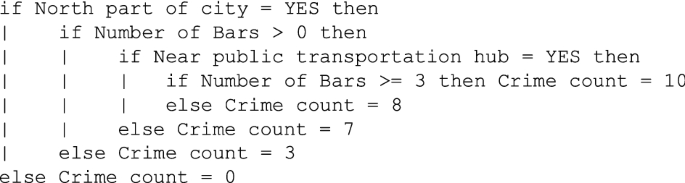
To predict a crime count at a particular location, one follows the splits in the data as described by the if–then statements, until one arrives at one of the 5 terminal nodes. This simple example shows that this city has a clear north–south divide: no crime is predicted to occur in the South of town, while in the North of town other predictor variables come into play. There, two variables predict crime: the presence of bars and whether the location is near a public transportation hub. A specific interaction is the best prediction of the counts of crime: if there are no bars present, the public transportation hub is not predictive of crime and 3 crimes are predicted. If bars are present but not near a public transportation hub the number of bars does not matter and 7 crimes are predicted to occur; but if the location is near a public transportation hub the number of bars matters (with one or two bars on the one hand, and three or more bars on the other hand), leading to a prediction of either 8 or 10 crimes.

The if–then statements are often visualized as a ‘tree’: starting at the top, the decisions branch out downwards until the final prediction is reached. Importantly, the tree is very easy to interpret by any audience: following such if–then rules is much easier than the standard parametric approach in this situation, parameter estimates of a Poisson regression model. The challenges are thus not in the interpretation but in the creation of the tree: for example, on which predictor variables should the data be partitioned (in every step) and at what value? And how many times should the data be partitioned, i.e. how many terminal nodes (or ‘leaves’) should the tree have? A variety of different techniques exist to deal with these challenges. For our purposes, it is important to note that a single tree is likely to overfit the data. That is, the tree will describe the predictors-response relationship too precisely for the given dataset; its predictive accuracy will not be high for new, out-of-sample data. In machine learning parlance, this means that a single tree will likely have low bias, but high variance.

RFs are one of the most popular ways to achieve low bias and low variance (although it’s impossible to minimize both at the same time, referred to in the literature as the ‘bias-variance tradeoff’). ‘Forest’ refers to the fact that a multitude of trees is created for the same dataset (often 500 trees in the default setting) and one averages the predictions over many individual trees to obtain a final prediction. It is called ‘random’ because each tree is grown for a bootstrap sample of the original data (i.e. a random sample with replacement) and using a random sample of all available predictor variables. Together, this leads to a model that has proved to be very effective in a wide variety of fields. For examples within criminology, Berk and Bleich (2013) show that RFs can accurately forecast recidivism, and Mohler and Porter (2018) use a RF model to generate short term place based crime predictions in a predictive policing challenge.

While RFs often have high predictive accuracy, they score low on interpretability: when the predictions of many trees are combined (that each can use different predictors and predict on different samples of the data), it is not possible to state explicitly one exact relationship between predictors and response. This raises a dilemma: what is more important, predictive accuracy, or interpretability? Scholars have different opinions on the dilemma. Breiman (2001a, b) argued that the point of a model is first and foremost to get accurate predictions, not interpretability. This sentiment is echoed in standard textbooks on predictive models or machine learning. Kuhn and Johnson (2013) give the example of someone selling his house (p.4): the seller does not care how a website estimates the selling value, only that the value is estimated correctly (as too high a price may drive away buyers while too low a price does not lead to the highest profit). On the other hand, the inability to assess why a forecasting model produced particular predictions might undermine its credibility (Ribeiro et al. 2016). This likely impedes the use of machine learning models in practice in the criminal justice system, even if they produce superior predictive performance over other models or methods (Bushway 2013; Ridgeway 2013).

In addition, identifying why a model predicted locations to be high (or low) crime might be informative for the formulation of effective problem-oriented policing approaches. A place predicted to be at high risk of robberies due to a high foot traffic area around public transportation would likely require a different approach than one around a high crime apartment complex (Braga et al. 1999; Guerette and Bowers 2009). To be clear: predictive models do not identify causal factors of crime, but variables that predict (i.e. are associated with) future crime.Footnote 5 That being said, predictive models have the potential to improve existing models by capturing complex, non-linear patterns (see Shmueli 2010 and Shmueli and Koppius 2011 for a general discussion of predictive models and their relationship with descriptive and explanatory models). While the outcomes of a predictive model should not be interpreted uncritically in a causal manner (Berk 2010), the factors most predictive of crime might give clues of the factors that cause crime. Additionally, such interpretations can give credibility to the models used, as they are often used in conjunction to identify high crime areas. Knowing why a place is predicted to be high crime can also serve as an important oversight mechanism to determine the legitimacy of the model and the data uses to arrive at the prediction (Ferguson 2017).

Fortunately, there exist a variety of techniques that can quantify the impact of the predictor variables across the ensemble of regression trees (e.g. Breiman 2000; Strobl et al. 2007). Recent advances allow one to reduce the complexity of machine learning models to simplified summaries that are easily interpretable (Molnar 2018). We illustrate three different interpretable summary techniques here; variable importance scores, average local effect plots, and Shapely value decompositions. While we provide a description of each technique in turn with the resulting graphics and tables when presenting results, we summarize these techniques here. Variable importance scores highlight how predictions are made less accurate when a particular variable is removed from the model. Average local effect plots show how, if you vary a variable, it changes the predicted value of the outcome (akin to a regression coefficient or a marginal effect). Shapely decompositions provide a reduced form description of how a particular variable contributes to a prediction for a particular observation.

Crime Data and Units of Analysis

The crime data under examination are reported interpersonal robberies from incident level data, geocoded to the address level. These incidents are available on the Dallas Open Data portal, https://www.dallasopendata.com. For analysis we split the data into a training set (from June 2014 through May 2016), and a testing set (from June 2016 through May 2018). This is to approximate how a police department would actually generate forecasts and identify areas to prioritize using historical information. Using the same data to both train the model and assess its accuracy would greatly over-estimate the accuracy of the model, hence the need to use a hold-out set of data (Berk 2008). There are a total of 6682 robberies in the training data, and 5931 robberies in the test data.

While other predictive policing applications are often oriented to generating very short term forecasts, often based on near repeat patterns (Mohler et al. 2011), problem-oriented approaches are not suitable for short-term forecasts in which the department is targeting a new location every week. Nor is long term urban planning, such as forecasting the future crime impact if a city zones for additional commercial locations. Thus we assess the predictive accuracy of the technique over a long period, effectively eliminating explanations of crime due to near-repeat patterns (Caplan et al. 2013a, b; Garnier et al. 2018; Ratcliffe et al. 2016; Taylor et al. 2015).Footnote 6 Given that micro level crime patterns tend to exhibit a strong amount of stability over time (Curman et al. 2014; Weisburd et al. 2004; Wheeler et al. 2016), forecasts over a long period of time are meaningful for police departments.

The spatial units of analysis are 200 by 200 feet grid cells over the city of Dallas. This distance was based on approximately half the size of the mean street segment in Dallas (which is 436 feet), which we rounded down to 200 feet for simplicity. Additionally as the crime data were geocoded using a street centerline file, only grid cells that were within 72 feet of a centerline were included. This eliminated one robbery that was over 200 feet away from a street centerline, and appeared to be geocoded using a rooftop method instead of a centerline method. Finally, the proportion of the grid cell covered by a 72-foot buffer of the street centerline was also included in the model. This acts as a local exposure variable: a grid cell that a street centerline only slightly passes through has less exposure than a grid cell that a street centerline runs down the middle of. This produces a total of 217,745 grid cells over the study area.

In subsequent random forest models, the centroid of the grid cell is used as a covariate as well. This allows the random forest model to potentially learn spatially varying coefficients (e.g. as an interaction between the x–y coordinates and the particular crime generator), as well as capture long term persistence in high crime areas.

Crime Generator Data

We have a total of eighteen different crime generator sources that are geocoded to the address level, and one that is based on polygon data (parks) (Brantingham and Brantingham 1993). Table 1 shows a description of each of the crime generator sources. These data sources are pulled from a variety of open data sources, commercial databases (such as Lexis Nexis, Reference USA), and local government GIS data files. “Appendix 1” provides a list of the variables, the original data source, and the associated standard industrial classification (SIC) code associated with each crime generator category.

Business locations were taken from three sources. The first was the street index database, originally compiled by the City Observatory (Cortright and Mahmoudi 2016). This database includes address level geocoded locations of stores, as well as their SIC code, which was used to classify the commercial locations into further thematic categories.

The different businesses and land uses in the street index database were further categorized into ad-hoc categories as to how they would be theoretically related to crime patterns at their exact location or in the vicinity. Ultimately breaking up the different businesses into different categories is somewhat arbitrary, but we have attempted to incorporate the many prior business categories as have been articulated in prior robbery research (Bernasco and Block 2011; Haberman et al. 2013; Kubrin and Hipp 2016). Table 1 displays those thematic categories and the total number of locations for each crime generator.

Larger business retailers include department stores (like JCPenney, Wal Mart, or Sears), hardware stores (like Home Depot), grocery stores, pharmacies (like CVS), and Dollar and craft stores. Smaller food and clothing stores include bakeries, herbal supplement stores, second hand stores, and clothing stores. While each type of commercial place affords more opportunities to commit an interpersonal robbery by having patrons coming and going, the latter group tend to be smaller in size, and thus will attract lower levels of foot traffic.

Eating and drinking places (aka restaurants and bars) are a common covariate predicting crime (Groff and Lockwood 2014). Movie theaters, amusement parks (like Six Flags), and recreation services (like concert halls) often involve large numbers of individuals congregating episodically within a small space (Kurland et al. 2014). The same is true of the final category: gyms, bowling alleys, museums, and hair salons, although these locations would be expected to have fewer individuals patronizing the services overall and individuals more consistently coming and going from the business over time.

The street index database was missing several businesses previously linked to robberies; gas stations (Bernasco and Block 2011), liquor stores (Block and Block 1995; Wheeler 2019b), and check cashing stores (Kubrin and Hipp 2016), so these are additionally added into the crime generator database. These business locations were obtained from commercial database venders Lexis Nexis and Reference USA. We include additional land use factors based on libraries (Groff and La Vigne 2001), public middle and high schools (Bernasco and Block 2011), light rail stations (Bernasco and Block 2011), apartments (Haberman et al. 2013), hospitals, motels, hotels (Clarke and Bichler-Robertson 1998), shopping malls (Brantingham and Brantingham 1993), mobile home parks (McCarty and Hepworth 2013), banks, and check-cashing stores (Kubrin and Hipp 2016). These locations are taken from various public data sources.Footnote 7

These point variables are coded for the risk terrain model (RTM) either using a density of the number of crime generators using a particular bandwidth (using a normal kernel), or as whether a crime generator is within a particular distance. The thresholds examined are 400 feet, 800 feet, and 1200 feet, which is consistent with other scholars work assessing the distance to which crime generators typically impact crime nearby (Groff and Lockwood 2014).Footnote 8 For parks we do not examine the number of parks within a particular distance, only the distance to the nearest park. We also do not examine the density of libraries, light rail stations, hospitals, and shopping malls. These variables are intentionally spread apart in Dallas, so one would only expect to find proximity effects for these crime generators. As is typically done for RTM models, we dichotomize those factors, receiving a value of 1 if within a particular distance band (and zero otherwise), or receives a 1 based on a z-score of above 2 for density factors. This dichotomization allows simpler interpretation of the relative risk of different factors on crime in the final model produced by RTM.

For the RF model, the density of crime generators using a 1000 foot bandwidth is included as an input (without dichotomizing the density). The RF model also includes the distance to the nearest crime generator in feet to predict the counts of crimes within the grid cell. This is because it is not necessary to create arbitrary thresholds for RFs to learn how far away that crime generator predicts crime, as RF automatically learns that function, as we will illustrate when we report the analysis.

Census Demographic Data

We also include census demographic data into the analysis. Although this is frequently not done at micro place based research (as the police have little control over census demographics), there are theories of crime that explain the spatial distribution of crime based on such demographic factors, most prominently social disorganization theory (Sampson 2012; Shaw and McKay 1969). While police cannot directly manipulate census demographics, they are likely important for understanding the antecedents of crime at micro places (Kim 2018), and thus should be taken into consideration for accurately predicting crime.

The demographic variables included in the analysis are taken from the 2014 five-year American Community Survey estimates at the block group level. The variables coded in the analysis are the proportion of families in poverty, the proportion of female headed households with children under eighteen, the proportion of individuals who have moved within the prior year, the proportion of individuals unemployed of those over sixteen and in the workforce, the proportion of the population that is non-Hispanic black, and the proportion of the population that is Hispanic. Additionally an index of ethnic heterogeneity is calculated using Simpson’s Index (Massey and Denton 1988), and this is based on the proportion of non-Hispanic White, black, and Hispanic population in a block group.Footnote 9 We also include the density of residential population. Grid cells within a block group were assigned that same proportional value (or density for the residential population). For grid cells that covered multiple block groups it was assigned the mean of those different demographics. When estimating the inter-item correlations of these variables at the block group level, they were always under 0.5, and so we do not consider the further step of creating a standardized index of social disorganization (Drawve et al. 2016; Miles et al. 2016).

The two main methods of comparison are Risk Terrain Modelling (Caplan and Kennedy 2011) and Random Forests (Breiman 2001a, b).

Risk Terrain Modeling

RTM uses a multiple step approach to select a limited number of variables that are used to explain the drivers of crime. The approach in RTM is as follows:

• Using a penalized Poisson regression where the coefficients are restricted to be positive, choose the model with the best L1 penalty given fixed small L2 costs.Footnote 10

• Based on those selected coefficients, use a step-wise model selection procedure that only selects one set of related variables (e.g. if two terms of an apartment within 400 feet, and an apartment within 800 feet are both selected by the prior step, this model selection step will only choose one of those variables).

• Repeat that same step for a Poisson and a negative binomial regression model, and subsequently choose the model with the lowest BIC.

While the underlying code for RTM is not made publicly available, we believe we have replicated the procedures (to the best of our ability) based on publicly available information (Caplan et al. 2013a, b; Kennedy et al. 2010; Kennedy et al. 2016).Footnote 11

Random Forests

As introduced previously, Random Forests are a machine learning technique that generates many trees and aggregates them into one prediction (Breiman 2001a, b). We use the R ranger library to estimate the RF models (Wright and Ziegler 2017).Footnote 12 These include all of the same predictor variables as in the RTM model, but instead of converted into 0/1 dummy variables are coded as the original distance to the nearest crime generator, or density of the crime generator within 1000 feet.

More Standard ‘Hot Spot’ Techniques

We also compare the accuracy of RTM and RFs to even more basic models. The first is a kernel density estimate calculated using the training data and generating the predictions. This is calculated using a normal kernel with a bandwidth of 600 feet. The other is using simply the count of crimes per grid cell in the training set to predict crime in the future.

Prior applications of assessing predictions for different hot spot techniques typically use the Predictive Accuracy Index (PAI) to assess the efficacy of those predictions (Drawve 2016; Drawve et al. 2016; Mohler and Porter 2018; Van Patten et al. 2009). The PAI metric can be written as:

where c equals the number of crimes in the predicted area given threshold t, and C is the total number of crimes. The denominator a equals the amount of area in the prediction given threshold t, and A equals the total study area. Or more simply the equation can be read as the proportion of crimes in a predicted area divided by the proportion of the area.

We consider two additional metrics, the Predictive Efficiency Index (PEI) (Hunt 2016), as well as the Recapture Rate Index (RRI). The PEI can be written as:

where PAIpPAIp is the PAI value obtained based on historical predictions, and PAImPAIm is the best possible PAI given the current data. Here we only make PEI comparisons among the same size area, and so the formula simply reduces to the proportion of crimes captured versus the proportion of crimes captured if the predictions were perfect. Thus PEI ranges in-between 0 and 1.

RRI was originally intended as a measure of accuracy of the predicted hot spots (Levine 2008). While prior applications have used the total number of previous crimes in the delimited hot spot area (Levine 2008: Van Patten et al. 2009), here we substitute the actual predictions made by the prediction method, and so RRI is simply the ratio of crimes predicted in a given threshold area t (using historical data) versus those observed.

Values closer to one for RRI suggest more accurate predictions, with values below 1 meaning the prediction method under-predicted the number of crimes that were subsequently observed, and values above 1 suggest the prediction method over-predicted the total number of crimes that were subsequently observed.

For a simplified example of the three metrics, in a city with 100 crimes and 100 areas, if one takes the top 10 areas (predicted using historical data), and in those top 10 areas there are 50 crimes, it would result in a PAI of (50/100)/(10/100)=0.5/0.1=5(50/100)/(10/100)=0.5/0.1=5. If the best possible 10 areas in the current data happen to capture a total of 75 crimes, the PEI would then be 50/75 = 2/3. If the predicted number of crimes in those top 10 areas was 65, the RRI would then equal 65/50 = 1.3.

The values for each metric will subsequently change depending on where the threshold number of areas is set. For RTM this threshold is often set at two standard deviations above the mean (i.e. a z-score prediction of over 2), which was similarly used in reference to kernel density estimation when the PAI metric was first introduced (Chainey et al. 2008; Drawve 2016). For the National Institute of Justice predictive policing challenge they fixed the threshold to a certain proportion of the area under study (Lee 2019; Mohler and Porter 2018). The latter may make more sense if one has a fixed number of resources to devote to hot spots policing, and so wants to allocate those fixed resources to the identified highest crime locations.

While fixing the threshold is necessary to make comparisons of PAI to predictive techniques that are binary, such as inside or outside of a nearest-neighbor hierarchical cluster (Chainey et al. 2008; Drawve 2016), it is not necessary for continuous model predictions, like that provided by RTM or RFs. We will subsequently provide graphical depictions of the PAI statistic along multiple potential thresholds. This will show the generalizability of the accuracy of the models no matter how a police department may decide to use the forecasts. For instance, one may decide to take the top 10 areas to focus on, another may highlight the top area in each police division, or another may decide to set the threshold based on the area needed to capture a specific number or proportion of crimes.

Accuracy of the Models

Table 2 displays the results of the predictions generated using the training data, but applied to the later test data. The table presents for each of the models under consideration, RTM, kernel density, RFs, and prior crimes, given particular fixed thresholds for areas. The table displays the cumulative number of interpersonal robberies captured within each of the thresholds, and also shows the estimated PAI. RTM tends to perform the worst out of each method, but performs similar in terms of predictive ability to that of a kernel density estimate. RFs outperforms both RTM and the kernel density estimate, but does not greatly outperform simply using prior crime counts as the prediction.

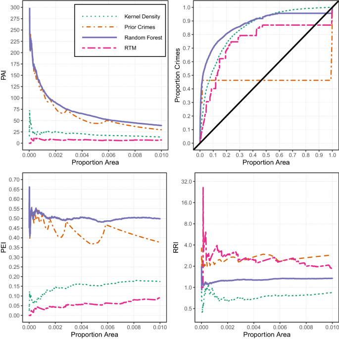
Setting fixed thresholds may be relevant if a police department has a pre-specified fixed number of areas that they want to focus a hot spots policing method on, and those fixed thresholds correspond to the total area they would be able to address. Because the thresholds reported in Table 2 are arbitrary, Fig. 1, top left corner, displays the PAI estimate for each of the different methods on the Y-axis for different proportions of the study area (up to 1% of the study area, which is over 2000 grid cells and over 3 square miles in total area) on the X-axis. One can see that regardless of the threshold chosen, RFs or using the prior crime counts outperforms RTM and KDE. PAI tends to decrease with the total number of areas, and each method has the highest PAI within just a small number of areas.Footnote 13

Fig. 1

Accuracy metrics for each of the different prediction models

Full size image

Interpreting the plot in the top right corner, it can be interpreted similarly to an ROC curve, but the Y-axis is weighted according to the cumulative number of crimes (Mohler and Porter 2018; Ohyama and Amemiya 2018). This again illustrates that simply using the prior crime counts provides reasonable predictions for future data at the very highest crime locations, as well as provides additional evidence for the law of crime concentration (Weisburd 2015). The top 5% of the predicted areas according to the RF model capture around 50% of the future robberies.

This is not surprising, as several analyses have identified long-term stability in crime patterns at micro places (Andresen et al. 2017; Curman et al. 2014; Weisburd et al. 2004; Wheeler et al. 2016), although such stability has been questioned in some recent work (Hipp and Kim 2017; Levin et al. 2017; Vandeviver and Steenbeek 2019). Examining the overall curve, the flat portion of the prior crimes (green line) is due to ties in the predictive metric. The long line accounts for areas that had zero crimes in the prior period, and so using prior crimes does not provide discrimination in how to choose those particular areas. The other predictors show more gradual curves, and all provide strong evidence that they are better than random predictions, with the RF prediction outperforming the kernel density and the RTM predictions. It also provides evidence that the other predictive models provide predictions for where crime might occur in the future, absent crimes observed in the past. But these predictions tend to be for overall low crime areas, so it is unclear if that result has much utility for a hot spots policing strategy.

The panel in the lower left depicts the PEI metric, again restricted to the top 1% of the area under study. It shows that RFs capture around 50% of the total crime compared to the best possible prediction, and again only slightly outperform the prior crime counts. It is a much improved metric over RTM and kernel density though, which tend to only capture around 5–20% of the same proportion of crimes.

The lower right panel depicts the RRI, and shows that RFs have the most accurate (closest to 1) values among the four predictors. This shows that RTM over-predicts the total number of crimes that would occur in the identified top predicted areas, as does using the prior crime counts. RFs over-predict only slightly, typically at a ratio of less than 1.5. KDE under-predicts the total amount of crime that would likely occur, because KDE spreads out predictions to areas where no prior crime occurred.Footnote 14

Interpreting Random Forests

Although the RF model has a higher predictive accuracy than RTM in this analysis, RTM has the potential advantage that it can be used to understand why locations are predicted to be risky. However, we will illustrate how to generate similar interpretations from the RF model using several recent advances in interpreting machine learning models.

Table 3 displays the overall variable importance score of each variable in the RF model, calculated by randomly permuting the feature (e.g. swapping the distance of the nearest liquor store with other grid cells, while keeping all other variables constant), and calculating the mean absolute error. The standard deviation of that error is calculated by repeating the process five times.Footnote 15 This allows one to rank variables by how important they are for prediction. For example, when removing the density of local apartment complexes from the prediction model, the mean absolute error increases by 3.45. This suggests that the absolute difference between the observed and predicted values over the sample are off by 3.45 crimes. This is a much larger error than when removing other variables from the model, such as Hotels, which result in a mean absolute error estimate of 1.56.

The most important variables for prediction are the density of several crime generators, including apartments, eating and drinking places, and larger business retailers. Population density also ranks highly as an important demographic feature, but the other demographic features are lower in feature importance relative to the crime generator factors. The x and y coordinates of the raster grid cells are within the middle of the list, and the proportion of the grid cell that is within 72 feet of a street centerline is the variable that provides the least improvement in predictability, but is still non-zero at a mean absolute error of slightly above one.

While these provide an intuitive ranking for the variables’ overall importance for prediction, they do not provide the equivalent interpretation of a regression coefficient.Footnote 16 Figure 2 displays accumulated local effect plots (Apley 2016; Molnar 2018) over increasing distances from train stops in the left hand panel, and in the right hand panel the effect of the proportion of population in poverty. These figures provide estimates more akin to marginal effects of the relationship between these predictor variables and robbery. Accumulated local effects are estimated by calculating the change in the predicted distribution when slightly varying X by a small amount, and then averaging that change over the entire observed distribution. For example, one calculates the predicted distribution when the value of X is replaced with 5 (holding all other variables in the sample at their observed values), call it p^x=5p^x=5. One then increases X to the value of 6, p^x=6p^x=6. One then takes the difference between the two predictions, p^x=6−p^x=5p^x=6−p^x=5, and then takes the average of those differences over the entire dataset. That average difference is the local effect when X = 6.Footnote 17 One then plots the cumulative sum of those local effects over a grid of X values, here determined by every percentile of X.

Fig. 2

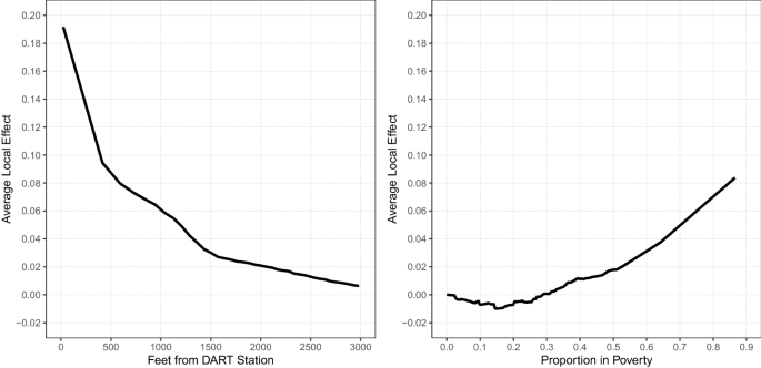
The average local effect of the distance to the nearest train station (left panel), and the proportion in poverty (right panel)

Full size image

The plot on the left shows how the distance to the nearest train station has a steeply decreasing function, although does not reach zero until after 3000 feet away. Previous work by Ratcliffe (2012) and Xu and Griffiths (2017) used change-point models to draw very similar effect plots. This approach provides complimentary evidence of similar decreasing effects, while not placing functional restrictions on the distance at which point those effects decay or are zero, which others have found to diffuse into larger areas (Groff 2014).

The plot on the right hand side illustrates the accelerating effect of extreme poverty. The effect hovers around zero for the range of 0–25% in poverty, shows a slight upward slope from 25 to 50%, but then appears to increase much more dramatically from 50% to over 80% in poverty. It has previously been hypothesized that concentrated disadvantage will have an accelerating rate on crime (Hipp and Yates 2011). Our findings are in line with that hypothesis, but it should be noted there are very few areas in Dallas with a concentration of over 50% poverty.

Accumulated local effect plots do not consider the interactions between those factors. Figure 3 displays the same accumulated local effect plot, but instead of fixing just one explanatory variable, varies two. Here we examine the interaction between the kernel density estimate of eating and drinking places on the X axis, and the proportion in poverty on the Y axis, and assign a color in the grid according to the average local effect when varying both of these factors. This plot thus captures hypothesized interactions between social disorganization and routine activity factors (Smith et al. 2000; Stucky and Ottensman 2009).Footnote 18 Figure 3 shows that the effect of both poverty and drinking places appear to be conditional on each other. That is, at low values of poverty, an increase in the number of drinking places does not have a large effect on crime. The same appears to be the case for increasing the proportion in poverty and holding the density estimate of drinking places at a low value. However, at high levels of poverty, increasing the number of drinking places appears to have the largest effect past a small threshold of drinking places nearby.

Fig. 3

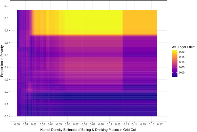
The average local effect when varying two variables, the density of eating and drinking places and the proportion of poverty within a census tract

Full size image

One final plot we examine is that of the predicted main drivers of crime in specific hotspots. Given that the RF model is non-linear over space, as well as includes a variety of interactions, this means that different identified hot spots may have different factors that contribute overall to crime. We do this by evaluating for individual observations a reduced model that assigns the predictive factors for a particular location via Shapley values (Shapley 1953; Molnar 2018). This provides, for each location, a decomposition of how each predictor variable contributes to the overall prediction.Footnote 19

This decomposition can help unpack not only why a particular place was predicted to be high crime, and thus improve understanding and trust of the model (Ribeiro et al. 2016), but can also identify the most relevant factors that the police should focus on when improvising problem-oriented approaches. So even if one cannot understand the model in its entirety, one can still incorporate the local model information into subsequent decision-making (Wachter, Mittelstadt, and Russell 2018).

Figure 4 displays several selected variables and how their contributions to crime vary over the space, similar in nature to geographically weighted regression (Cahill and Mulligan 2007; Fotheringham et al. 2003; Graif and Sampson 2009; Light and Harris 2012; Weisburd et al. 2014). In the top left corner, the contribution of population density is mostly limited to the northern parts of Dallas in more residential neighborhoods. The effect of the distance to the nearest gas station (top right) shows a very different pattern, contributing to hot spots more frequently in the southeastern part of the city. The bottom right map illustrates that while apartment complexes are one of the strongest predictors according to the variable importance score, there effect is most pronounced in the northeastern part of the city and much less elsewhere. This promotes the idea of Eck et al. (2007) that certain facilities are not monolithic in their contribution towards crime, and the local contribution scores reflect this reality. Finally, the map in the lower right displays the effect of eating and drinking places, which has a larger contribution at a hot spot in the northwestern part of Dallas but only sparse contributions otherwise. These locally interpretable scores aid problem-oriented approaches to specific hot spots, as opposed to attributing crime to specific factors uniformly across the entire study area. For example, one could make an interactive map of the output, and identify the particular predictors that contribute to risk scores at a particular high crime predicted area (including specific crime generators themselves).

Fig. 4

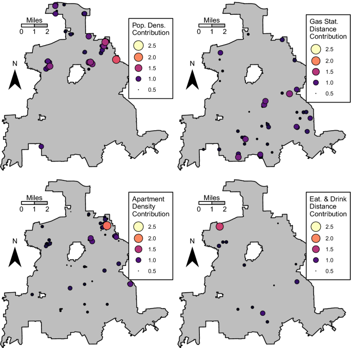
Contribution of different risk factors to predicted crime counts over space. Factors are calculated using Shapley value regression, and locations with a risk factor of over 0.5 are shown

Full size image

Machine learning models have a variety of potential applications towards policing, such as identifying chronic offenders (Wheeler et al. 2019), linking offenses committed by the same offender (Chohlas-Wood and Levine 2019; Reich and Porter 2015), as well as producing spatial predictions (Hipp et al. 2017; Mohler and Porter 2018). While the accuracy of using machine learning models has been established across various applications in criminal justice (Berk and Bleich 2013; Mohler and Porter 2018), their black box nature comes at a potential loss in interpretability. We illustrate how to generate interpretable model summaries that can be used to decipher this predictive importance for crime at micro places.

The RF model does not rely on a pre-specified set of linear and additive relationships that need to be specified by the researcher at the onset of the study. Thus it relies on fewer assumptions than typical regression models. While this comes at the cost of increased complexity, we illustrate here how interpretable model summaries can aid in assessing the predictions of different hypotheses regarding interaction and threshold effects. Identifying those interactions and non-linear effects are often of interest to test different criminological hypotheses, as well as important to understand when formulating localized problem oriented approaches to tackle crime.

While we focus on RFs in this particular evaluation, we do not discount the ability of other machine learning models such as generalized boosted models or neural networks to accurately predict crime at micro places based on the same inputs used here (see e.g. Rummens et al. 2017). We believe RFs are flexible enough to identify the various non-linear and spatially varying functions that criminologists have previously hypothesized (Wang et al. 2016), but RFs should not be considered the ultimate model all researchers should use, nor should these results be taken as sacrosanct that RFs will always outperform other models used to predict crime at micro places.

We show several different summaries that illustrate common hypotheses in criminal justice research. We show an increasing effect of poverty on crime (Hipp and Yates 2011), as well as a non-linear distance decay effect of nearby crime generators (Ratcliffe 2012; Xu and Griffiths 2017) using average local effect plots. Additionally we show an interaction effect between poverty and the density of nearby drinking places using average local effect plots varying two variables (Smith et al. 2000; Stucky and Ottensman 2009). We show the spatially varying relationships between different crime generators and demographic factors over the city of Dallas using a local Shapley decomposition of how different factors increase crime. This can replace geographically weighted regression models (Cahill and Mulligan 2007; Fotheringham et al. 2003; Graif and Sampson 2009; Light and Harris 2012; Weisburd et al. 2014), which can often be inaccurate (Wheeler and Waller 2009). It also conforms to the hypothesis that not all places monolithically contribute to crime (Eck et al. 2007). Thus such simple model summaries actually better facilitate local problem-oriented police approaches in particular hot spots, instead of attributing crime to single factors across the entire study area (Caplan and Kennedy 2011).

While we believe the use of RFs can increase the accuracy of micro-place crime predictions, it is not a panacea. The analysis we conduct here is predictive: any causal inferences made based on this analysis are likely weak compared to experimental or quasi-experimental designs. For a police department identifying hot spots of crime and assessing potential putative factors that contribute to those hot spots this is a limitation they will likely have to live with in practice. But for researchers suggesting policy interventions, the use of machine learning models does not circumvent the need for stronger research designs to assess causality and likely changes in crime in response to different interventions.

One particular confound that we would like to emphasize here is the lack of using prior crimes to predict future crimes. Such near repeat patterns are the basis for self-exciting prediction models that have been used in prior predictive policing applications (Mohler et al. 2011, ; 2015). In this paper we focused on long-term crime trends, and therefore chose to not include near repeat crime into our predictive model (Taylor et al. 2015). However, near repeat factors can be incorporated into RF models by predicting crimes over shorter time periods and including factors such as the number of nearby crimes within a short time period (Mohler and Porter 2018). This opens up new research avenues using our predictive model: to investigate the extent to which certain place based characteristics interact with crime to create greater or lesser risk for near repeat crime events (Caplan et al. 2013a, b; Garnier et al. 2018; Moreto et al. 2014; Piza and Carter 2018).

Given the long term predictability of crime at micro-places however (Andresen et al. 2017; Curman et al. 2014; Weisburd et al. 2004; Wheeler et al. 2016), we believe an approach that identifies long-term crime hot spots and decomposes the effects to different local crime generators and demographic factors, can be successfully incorporated into problem-oriented hot spots policing strategy. While prior short term hot spots approaches have yielded successful interventions (Mohler et al. 2015; Ratcliffe et al. 2020), the majority of the research on effective hot spot strategies on crime point to more long term, problem solving approaches (Braga et al. 2014). Thus even if one can effectively predict crime at micro places, it may be that long term strategies to reduce crime at places is the more effective approach for police departments to take.

This is important to consider in relation to another of the findings of the study; that simply using the prior counts of crime provides very similar predictions in terms of accuracy to those of RFs, of which both are much more effective in identifying high crime areas than RTM or kernel density estimation. This is likely due to the historical persistence of crime at micro place hot spots (Curman et al. 2014; Weisburd et al. 2004; Wheeler et al. 2016). The majority of prior applications of examining the accuracy of different prediction methods do not test whether the predictions are more accurate relative to simply prior crime counts (Caplan and Kennedy 2011; Drawve 2016; Chainey et al. 2008; Levine 2008). Simple metrics, such as counting up the number of crimes in the prior three years, seem to be effective in identifying hot spots of crime to target, especially relative to human based judgements (Macbeth and Ariel 2019; Ratcliffe and McCullagh 2001). However, the RF model has very similar predictive accuracy while also giving information on predictor variables that in turn may provide clues for the potential causes of crime at micro places. In addition, the illustrated interpretable model summaries based on this inputted factors can inform future urban planning, especially in regards to predicting the potential effects that increasing commercial development may have on future crime patterns.

The spatial models presented in this paper myopically focus on spatial factors that contribute to crime, and ignore individual human elements. It may be the case that identifying hot spots of crime, and then identifying chronic offenders to focus on within those hot spots is an effective strategy (Groff et al. 2015; Uchida and Swatt 2013). The current approach of this paper—as with the majority of crime and place based research—does not aid in accomplishing that objective. Note however, that incorporating such individual aspects into the predictive models comes with additional concerns of disparate impact that can occur as the result of predictive models (Ridgeway 2018), although such concerns are not entirely absent from spatial predictive models either (Brayne 2017; Harcourt 2007; Kochel 2011; Wheeler 2019a). Interpretable model summaries can effectively address how different factors contribute to the prediction, even if they cannot depict the entire complexity of a machine learning model (Wachter et al. 2018). This by itself is an important step to audit and fully understand a predictive model in practice (Ribeiro et al. 2016).

Another limitation is that while here we incorporate a raster-based approach, it is possible that different types of spatial units—e.g., street segments and intersections—may provide either better forecasts (Rosser et al. 2017) or more relevant prediction metrics (Drawve and Wooditch 2019). Given that street segments and intersections are currently very popular micro place spatial units to generate models (Andresen et al. 2017; Braga et al. 2010; Steenbeek and Weisburd 2016; Weisburd et al. 2004; Wheeler et al. 2016), it might also be the case that address-level predictions provide more easily actionable problem oriented strategies (Deryol et al. 2016; Eck et al. 2007).

The RF model illustrated here can be extended to such vector units, so ultimately using raster units is only a critique of the current analysis, not of the technique in-and-of-itself. Police departments creating the forecasts will need to make operational decisions about what, where, and when exactly to forecast that best aids with their particular policing strategy (Haberman 2017). We believe the RF model presented here can be used flexibly to produce such forecasts. With the interpretable model summaries they can not only produce accurate forecasts for crime at micro places, but can also be used to understand potential drivers of crime at those micro places. While simply knowing those potential causal factors still does not directly imply particular place based strategies to mitigate crime (Ridgeway 2018; Weisburd and Telep 2014), they no doubt inform problem-oriented policing strategies, as well as offer evidence for or against different theories of interest to crime and place based researchers.

Interpretation of those factors that potentially contribute to crime requires careful consideration. While random forests can provide accurate forecasts, the technique does not prevent overfitting of the effects of different crime generators, nor does it provide causal inferences.Footnote 20 Take for example a city that has long-standing historical persistence on high crime areas around commercial areas (Schmid 1926; Shaw and McKay 1969). These are also areas that by construction (due to zoning laws), have a higher proportion of commercial crime generator locations. Thus the model may learn to apportion variance to those local crime generators, but the relationship may be spurious due to the long standing historical consistency of high crime areas (Kelly 2019). This is ultimately a critique of all work that uses cross-sectional correlations to identify factors that contribute to crime, whether they be predictive or inferential in nature. As such, the suggestion of using random forests to uncover those non-linear effects and interactions is only a marginal improvement over that past work.

One way future research could take this into account is to incorporate spatial cross-validation (Brenning 2012; Roberts et al. 2017), which prevents the model from overfitting to local circumstances. Unfortunately, this is not consistent with the attempt to learn spatially varying effects, e.g. a bar in one area of the city may have a large effect, and another may have no effect on crime (Eck et al. 2007). Such local variation in effects will always be confounded with long-term historical persistence of hot spots as a potential explanation.

The current random forest technique (or any machine learner) simply partitions the observed variance in high crime areas to factors that you put in. As such it could be considered a tautology, in that it will only ever say a particular crime generator contributes to the local crime factors that the researcher has already pre-determined are relevant—it cannot tell the analyst what factors to put into the machine to begin with. While we believe such a partition is useful to researchers and practitioners, in that it reduces a very high dimension of potential correlates into a reduced form summary, it can lead one astray in presuming too much on the nature of crime at local places.

Data and code to replicate the results can be downloaded from https://www.dropbox.com/sh/b3n9a6z5xw14rd6/AAAjqnoMVKjzNQnWP9eu7M1ra?dl=0.

1. 1.

   For more discussion about self-exciting point processes, see the full issue of Statistical Science volume 33(3) with several commentaries on Reinhart (2018) as well as a rejoinder responding to these commentaries.

2. 2.

   Why a grid cell is estimated to be high risk should not imply that the highlighted covariates are then a causal explanation for crime. The identified land use features correlate with crime and hopefully predict better than chance where future crime will occur, but one should not infer a causal mechanism.

3. 3.

   Even these are not exclusive of how one may measure the impact of a crime generator. Another common approach is to estimate the number of generators nearby, where nearby is either a specific buffer distance, or determined via adjacency of some aggregate unit (Bernasco and Block 2011; Haberman and Ratcliffe 2015; Murray and Roncek 2008; Wheeler 2019b).

4. 4.

   See the related discussion on how encoding of the interactions in Deryol et al. (2016) was innapropriate to actually estimate interaction effects (Reinhart 2016).

5. 5.

   Thus a clear difference of predictive models as compared to explanatory models is that the goal is to predict (out-of-sample) crime. That is, the main goal is not to derive causal hypotheses from a causal theoretical model and test these using empirical data. Instead, the goal of predictive models is to predict new or future observations (e.g. point estimates, interval predictions, or rankings).

6. 6.

   The most accurate forecasting models are often models that combine different machine learning methods that together predict crime. Using the same logic, our paper is not antagonistic of self-exciting point process models (Mohler et al. 2011). Instead, we see the value of using such methods to predict short-to-medium crime occurrence, while our models can be used to predict medium-to-long term crime trends and also allow for crime predictions in ‘what-if’ scenarios.

7. 7.

   Given these crime generator variables come from various sources, they are not uniformly prior to the crime counts used in the research. While the street index database is based on 2014 data, many of the other factors are based on more recent data collections. We do not believe it represents a large threat to the findings though, as many of the factors are historically stable due to long standing zoning laws in Dallas (Fischel 2015).

8. 8.

   Given the large size of the variable set, we do not test for half block increments of 200 feet. Caplan et al. (2013a, b) suggest to limit the variable count to 100 or less.

9. 9.

   Simpson’s Index for a block group equals (pwhite)2+(pblack)2+(pHispanic)2(pwhite)2+(pblack)2+(pHispanic)2 where p represents the proportion of that particular racial group.

10. 10.

    The fixed L2 costs are one aspect we are not able to replicate given public descriptions. We considered two L2 costs of 1 and 5 in this step. To determine the best L1 penalty we use cross-validation, consistent with the code provided in Kennedy et al. (2016).

11. 11.

    We conduct RTM analysis that both excludes demographic factors as well includes demographic factors. The models that included demographic factors were much more accurate than those that did not along all of the metrics we evaluate, so we only report the RTM model that includes demographic factors into the model selection process. “Appendix 2” lists the final produced RTM model.

12. 12.

    The default settings in the ranger implementation are used, i.e. the number of trees is set to 500, and resampling is done with replacement.

13. 13.

    Several of the sawtooth or flat line patterns are due to how we treat prediction ties in Fig. 1, most noticeable for the plot in the top right and the plot in the bottom left. Here we present the worst case scenario, sorting the predictions in descending order, and the future crimes in ascending order. This is typically how ROC plots are displayed (Davis and Goadrich 2006), and so it is similarly appropriate for these metrics as well.

14. 14.

    To calculate the expected number of crimes per the kernel density estimate we multiplied the intensity kernel density value by the area of the grid cell, thus getting an expected number of crimes per grid cell.

15. 15.

    Because of the size of the dataset and number of variables, to calculate this we selected a stratified sample of 2000 cases within 10 strata (so overall 20,000 cases). The strata were defined by the crime counts in the cells, with ties broken by the predicted number of crimes.

16. 16.

    The correct predictive interpretation of a regression coefficient is a comparison between grid cells: how much does crime differ, on average, when comparing two groups of grid cells that differ by 1 in the relevant predictor while being identical in all the other predictors. Only under stringent assumptions can one make a counterfactual interpretation of changes within grid cells: the expected change in crime in that grid cell caused by adding 1 to the relevant predictor, while leaving all the other predictors in the model unchanged (see Gelman and Hill 2006, p. 34). With perhaps a few exceptions, all studies cited in this paper are of the former type.

17. 17.

    Such average predictive comparisons can be used to understand any complicated regression model, not just random forests, see Gelman and Pardoe (2007) for a similar procedure. It is also very similar in nature to the local derivatives reported in Hipp et al. (2017).

18. 18.

    An additional way to examine interactions are via Friedman’s H statistic (Friedman and Popescu 2008; Wang et al. 2016).

19. 19.

    For example, a location may have a predicted 5 crimes in the area: the distance to the nearest liquor store contributes 3.6 to that prediction, while the proportion in poverty contributes 1.3, and the rest of the predictor variables combine for the additional 0.1 predicted crimes (including factors that potentially decrease crime).

20. 20.

    We have provided supplementary random forest models to illustrate this confounding in “Appendix 3”. One is a model only using the exact same variables as the RTM model (the binary indicators and the demographic factors), and another using only the XY coordinates of the grid cell. While the model presented in the paper outperforms either, random forests trained on those different subsets of data still provide excellent future predictions.

Affiliations

1. Data Scientist, HMS, 5615 High Point Dr #100, Irving, TX, 75038, USA

   Andrew P. Wheeler

2. Netherlands Institute for the Study of Crime and Law Enforcement, Amsterdam, The Netherlands

   Wouter Steenbeek

Corresponding author

Correspondence to Andrew P. Wheeler.

Publisher's Note

Springer Nature remains neutral with regard to jurisdictional claims in published maps and institutional affiliations.

Commentary expressed within the manuscript do not represent the views of HMS.

Appendix 1: Crime Generator Data Source and SIC Code Classifications

This appendix provides additional information on the source of the crime generator data, as well as the SIC codes associated with different business categories. Store Front Index point data for Dallas can be downloaded from https://github.com/dillonma/storefrontindex. Public data downloads are mostly taken from https://gis.dallascityhall.com/shapefileDownload.aspx or http://gis.dallascityhall.com/wwwgis/rest/services. Texas schools are taken from https://schoolsdata2-tea-texas.opendata.arcgis.com/. The only reason check cashing stores are taken from Reference USA as opposed to Lexis Nexis is my local library cut the service for Lexis Nexis. The storefront data are businesses as of 2015. The rest of datasets were collected in 2018.

See Tables 4 and 5.

Appendix 2: RTM Predicted Model

See Table 6.

Appendix 3: Additional Random Forest Model Performance Metrics

See Fig. 5.

Fig. 5

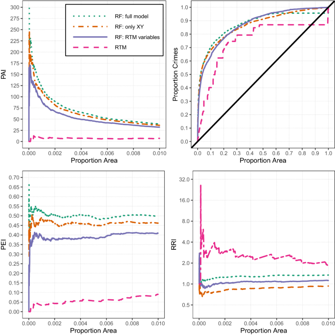
Predictive statistics for supplementary random forest models. “RF: Full Model” is the same model as that presented in the main manuscript for Random Forests, and “RTM” is the original RTM model in the main manuscript. “RF: only XY” is a random forest model trained with only the XY coordinates. “RF: RTM variables” is a random forest model trained with the exact same variables input into RTM (dummy variables for distance and density, plus continuous variables for demographic characteristics)

Full size image

Reprints and Permissions

References

Andresen MA (2006) Crime measures and the spatial analysis of criminal activity. Brit J Criminol 46:258–285
Andresen MA, Jenion GW (2008) Crime prevention and the science of where people are. Crim Justice Policy Rev 19:164–180
Andresen MA, Curman AS, Linning SJ (2017) The trajectories of crime at places: understanding the patterns of disaggregated crime types. J Quant Criminol 33:427–449
Apley DW (2016) Visualizing the effects of predictor variables in black box supervised learning models. arXiv:1612.08468
Barnum JD, Caplan JM, Kennedy LW, Piza EL (2017) The crime kaleidoscope: a cross-jurisdictional analysis of place features and crime in three urban environments. Appl Geogr 79:203–211
Berk R (2008) Forecasting methods in crime and justice. Ann Rev Law Soc Sci 4:219–238
Berk R (2010) What you can and can’t properly do with regression. J Quant Criminol 26:481–487
Berk R (2013) Algorithmic criminology. Secur Inform 2(1):5
Berk R, Bleich J (2013) Statistical procedures for forecasting criminal behavior. Criminol Public Policy 12:513–544
Bernasco W, Block RL (2011) Robberies in Chicago: a block-level analysis of the influence of crime generators, crime attractors, and offender anchor points. J Res Crime Delinq 48:33–57
Bien J, Taylor J, Tibshirani R (2013) A lasso for hierarchical interactions. Ann Stat 41:1111–1141
Block RL, Block CR (1995) Space, place and crime: hot spot areas and hot places of liquor-related crime. Crime Prev Stud 4:145–184
Boessen A, Hipp JR (2018) Parks as crime inhibitors or generators: examining parks and the role of their nearby context. Soc Sci Res 76:186–201
Boivin R, Felson M (2018) Crimes by visitors versus crimes by residents: the influence of visitor inflows. J Quant Criminol 34:465–480
Bowers KJ, Johnson SD, Pease K (2004) Prospective hot-spotting: the future of crime mapping? Br J Criminol 44:641–658
Braga AA, Weisburd DL, Waring EL, Mazerolle LG, Spelman W, Gajewski F (1999) Problem-oriented policing in violent crime places: a randomized controlled experiment. Criminology 37:541–580
Braga AA, Papachristos AV, Hureau DM (2010) The concentration and stability of gun violence at micro places in Boston, 1980–2008. J Quant Criminol 26:33–53
Braga AA, Papachristos AV, Hureau DM (2014) The effects of hot spots policing on crime: an updated systematic review and meta-analysis. Justice Q 31:633–663
Brantingham PL, Brantingham PJ (1993) Nodes, paths and edges: considerations on the complexity of crime and the physical environment. J Environ Pyschol 13:3–28
Brayne S (2017) Big data surveillance: the case of policing. Am Soc Rev 82:977–1008
Breiman L (2000) Randomizing outputs to increase prediction accuracy. Mach Learn 40(3):229–242
Breiman L (2001a) Random forests. Mach Learn 45:5–32
Breiman L (2001b) Statistical modeling: the two cultures. Stat Sci 16:199–231
Brenning A (2012) Spatial cross-validation and bootstrap for the assessment of prediction rules in remote sensing: the R package sperrortest. In: IEEE international geoscience and remote sensing symposium, July
Bushway SD (2013) Is there any logic to using logit? Finding the right tool for the increasingly important job of risk prediction. Criminol Public Policy 12:563–567
Cahill M, Mulligan G (2007) Using geographically weighted regression to explore local crime patterns. Soc Sci Comput Rev 25:174–193
Caplan JM, Kennedy LW (2011) Risk terrain modelling: brokering criminological theory and GIS methods for crime forecasting. Justice Q 28:360–381
Caplan JM, Kennedy LW, Piza EL (2013a) Joint utility of event-dependent and environmental crime analysis techniques for violent crime forecasting. Crime Delinq 59:243–270
Caplan JM, Kennedy LW, Piza EL, with a chapter contribution by Heffner J (2013b) Risk terrain modeling diagnostics utility USER MANUAL. Rutgers Center on Public Security. http://www.rutgerscps.org/uploads/2/7/3/7/27370595/rtmdxusermanual_final_caplankennedypiza.pdf. Accessed 4 Oct 2019
Chainey S, Thompson L, Uhlig S (2008) The utility of hotspot mapping for predicting spatial patterns of crime. Secur J 21:4–28
Chohlas-Wood A, Levine ES (2019) A recommendation engine to aid in identifying crime patterns. Inf J Appl Anal 49:154–166
Clarke RV, Bichler-Robertson G (1998) Place managers, slumlords, and crime in low rent apartment buildings. Secur J 11:11–19
Cohen LE, Felson M (1979) Social change and crime rate trends: a routine activity approach. Am Sociol Rev 44:588–608
Cortright J, Mahmoudi D (2016) City report: the storefront index. City Observatory. http://cityobservatory.org/wp-content/uploads/2016/04/Storefront_Index_April_2016.pdf. Accessed 3 May 2019
Curman AS, Andresen MA, Brantingham PJ (2014) Crime and place: a longitudinal examination of street segment patterns in Vancouver, BC. J Quant Criminol 31:127–147
Davis J, Goadrich M (2006) The relationship between precision-recall and ROC curves. In: Proceedings of the 23rd international conference on machine learning
Deryol R, Wilcox P, Logan M, Wooldredge J (2016) Crime places in context: an illustration of the multilevel nature of hotspot development. J Quant Criminol 32:305–325
Drawve G (2016) A metric comparison of predictive hot spot techniques and RTM. Justice Q 33:369–397
Drawve G, Barnum JD (2015) Place-based risk factors for aggravated assault across police divisions in Little Rock, Arkansas. J Crime Justice 41:173–192
Drawve G, Wooditch A (2019) A research note on the methodological and theoretical considerations for assessing crime forecasting accuracy with the predictive accuracy index. J Crim Justice 64:101625
Drawve G, Moak SC, Berthelot ER (2016a) Predictability of gun crimes: a comparison of hot spot and risk terrain modelling techniques. Police Soc 26:312–331
Drawve G, Thomas SA, Walker JT (2016b) Bringing the physical environment back into neighborhood research: the utility of RTM for developing an aggregate neighborhood risk of crime measure. J Crim Justice 44:21–29
Eck J, Chainey S, Cameron J, Wilson R (2005) Mapping crime: understanding hotspots. National Institute of Justice. Washington, D.C.
Eck JE, Clarke RV, Guerette RT (2007) Risky facilities: crime concentration in homogenous setes of establishments and facilities. Crime Prev Stud 21:225–264
Efron B, Hastie T (2016) Computer age statistical inference, vol 5. Cambridge University Press, Cambridge
Ferguson AG (2017) The rise of big data policing: surveillance, race, and the future of law enforcement. New York University Press, New York
Fischel WA (2015) Zoning rules!: the economics of land use regulation. Lincoln Institute of Land Policy, Massachusetts
Fotheringham AS, Brunsdon C, Charlton M (2003) Geographically weighted regression: the analysis of spatially varying relationships. Wiley, West Sussex
Friedman JH, Popescu BE (2008) Predictive learning via rule ensembles. Ann Appl Stat 2:916–954
Garnier S, Caplan JM, Kennedy LW (2018) Predicting dynamical crime distribution from environmental and social influences. Front Appl Math Stat 4:13
Gelman A, Hill J (2006) Data analysis using regression and multilevel/hierarchical models. Cambridge University Press, Cambridge
Gelman A, Pardoe I (2007) Average predictive comparisons for models with nonlinearity, interactions, and variance components. Sociol Methodol 37:23–51
Gerell M (2018) Bus stops and violence, are risky places really risky? Eur J Crim Policy Res 24:351–371
Graif C, Sampson RJ (2009) Spatial heterogeneity in the effects of immigration and diversity on neighborhood homicide rates. Homicide Stud 13:242–260
Groff ER (2014) Quantifying the exposure of street segments to drinking places nearby. J Quant Criminol 30:527–548
Groff ER, La Vigne NG (2001) Mapping an opportunity surface of residential burglary. J Res Crime Delinq 38:257–278
Groff ER, La Vigne NG (2002) Forecasting the future of predictive crime mapping. Crime Prev Stud 13:29–57
Groff ER, Lockwood B (2014) Criminogenic facilities and crime across street segments in Philadelphia: uncovering evidence about the spatial extent of facility influence. J Res Crime Delinq 51:277–314
Groff ER, Ratcliffe JH, Haberman CP, Sorg ET, Joyce NM, Taylor RB (2015) Does what police do at hot spots matter? The Philadelphia policing tactics experiment. Criminology 53:23–53
Guerette RT, Bowers KJ (2009) Assessing the extent of crime displacement and diffusion of benefits: a review of situational crime prevention evaluations. Criminology 47:1331–1368
Haberman CP (2017) Overlapping hot spots? Examination of the spatial heterogeneity of hot spots of different crime types. Criminol Public Policy 16:633–660
Haberman CP, Ratcliffe JH (2015) Testing for temporally differentiated relationships among potentially criminogenic places and census block street robbery counts. Criminology 53:457–483
Haberman CP, Groff ER, Taylor RB (2013) The variable impacts of public housing community proximity on nearby street robberies. J Res Crime Delinq 50:163–188
Harcourt BE (2007) Against prediction: profiling, policing, and punishing in an actuarial age. University of Chicago Press, Chicago
Hastie T, Tibshirani R, Friedman J (2009) The elements of statistical learning: prediction, inference and data mining. Springer, New York
Hipp JR (2016) General theory of spatial crime patterns. Criminology 54:653–679
Hipp JR, Boessen A (2013) Egohoods as waves washing across the city: a new measure of “neighborhoods”. Criminology 51:287–327
Hipp JR, Kim Y (2017) Measuring crime concentration across cities of varying sizes: complications based on the spatial and temporal scale employed. J Quant Criminol 33:595–632
Hipp JR, Steenbeek W (2016) Types of crime and types of mechanisms: what are the consequences for neighborhoods over time? Crime Delinq 62(9):1203–1234
Hipp JR, Yates DK (2011) Ghettos, thresholds, and crime: does concentrated poverty really have an accelerating increasing effect on crime? Criminology 49:955–990
Hipp JR, Kane K, Kim JH (2017) Recipes for neighborhood development: a machine learning approach toward understanding the impact of mixing in neighborhoods. Landsc Urban Plan 164:1–12
Hipp JR, Bates C, Lichman M, Smyth P (2019) Using social media to measure temporal ambient population: does it help explain local crime rates? Justice Q 36:718–748
Hunt J (2016) Do crime hot spots move? Exploring the effects of the modifiable areal unit problem and modifiable temporal unit problem on crime hot spot stability. Dissertation, American University
Johnson SD (2014) How do offenders choose where to offend? Perspectives from animal foraging. Legal Criminol Psychol 19:193–210
Johnson SD, Summers L, Pease K (2009) Offender as forager? A direct test of the boost account of victimization. J Quant Criminol 25:181–200
Jones RW, Pridemore WA (2019) Toward an integrated multilevel theory of crime at place: routine activities, social disorganization, and the law of crime concentration. J Quant Criminol 35:543–572
Kelly M (2019) The standard errors of persistence. SSRN. https://papers.ssrn.com/sol3/papers.cfm?abstract_id=3398303. Accessed 4 Oct 2019
Kennedy LW, Caplan JM, Piza E (2010) Risk clusters, hotspots, and spatial intelligence: risk terrain modelling as an algorithm for police resource allocation. J Quant Criminol 27:339–362
Kennedy LW, Caplan JM, Piza E, Buccine-Schraeder H (2016) Vulnerability and exposure to crime: applying risk terrain modeling to the study of assault in Chicago. Appl Spat Anal Policy 9:529–548
Kim YA (2018) Examining the relationship between the structural characteristics of place and crime by imputing census block data in street segments: is the pain worth the gain? J Quant Criminol 34:67–110
Kim YA, Hipp JR (2020) Street egohood: an alternative perspective of measuring neighborhood and spatial patterns of crime. J Quant Criminol 36:29–66
Kochel TR (2011) Constructing hot spots policing: unexamined consequences for disadvantaged populations and for police legitimacy. Crim Justice Policy Rev 22:350–374
Kubrin CE, Hipp JR (2016) Do fringe banks create fringe neighborhoods? Examining the spatial relationship between fringe banking and neighborhood crime rates. Justice Q 33:755–784
Kuhn M, Johnson K (2013) Applied predictive modeling, vol 26. Springer, New York
Kurland J, Johnson SD, Tilley N (2014) Offenses around stadiums: a natural experiment on crime attraction and generation. J Res Crime Delinq 51:5–28
Lee YJ, O SH, Eck JE (2019) A theory driven algorithms for real-time crime hot spot forecasting. Police Q
Levin A, Rosenfeld R, Deckard M (2017) The law of crime concentration: an application and recommendations for future research. J Quant Criminol 33:635–647
Levine N (2008) The “Hottest” part of a hotspot: commentary on “The utility of hotspot mapping for predicting spatial patterns of crime”. Secur J 21:295–302
Light MT, Harris CT (2012) Race, space, and violence: exploring the spatial dependence in structural covariates of white and black violent crime in US counties. J Quant Criminol 28:559–586
Loftin C (1986) Assaultive violence as a contagious social process. Bull N Y Acad Med 62:550–555
Macbeth E, Ariel B (2019) Place-based statistical versus clinical predictions of crime hot spots and harm locations in Northern Ireland. Justice Q 36:93–126
Malleson N, Andresen MA (2015) The impact of using social media data in crime rate calculations: shifting hot spots and changing spatial patterns. Cartogr Geogr Inf Sci 42:112–121
Massey DS, Denton NA (1988) The dimensions of residential segregation. Soc Forces 67:281–315
McCarty WP, Hepworth DP (2013) Mobile home parks and crime: does proximity matter? J Crime Justice 36:319–333
Miles JN, Weden MW, Lavery D, Escarce JJ, Cagney KA, Shih RA (2016) Constructing a time-invariant measure of the socio-economic status of U.S. census tracts. J Urban Health 93:213–232
Mohler G (2014) Marked point process hotspot maps for homicide and gun crime prediction in Chicago. Int J Forecast 30(3):491–497
Mohler GO, Porter MD (2018) Rotational grid, PAI-maximizing crime forecasts. Stat Anal Data Min 11:227–236
Mohler GO, Short MB, Brantingham PJ, Schoenberg FP, Tita GE (2011) Self-exciting point process modeling of crime. J Am Stat Assoc 106:100–108
Mohler GO, Short MB, Malinowski S, Johnson M, Tita GE, Bertozzi AL, Brantingham PJ (2015) Randomized controlled field trials of predictive policing. J Am Stat Assoc 110:1399–1411
Molnar C (2018) Interpretable machine learning: a guide for making black box models explainable. https://christophm.github.io/interpretable-ml-book/. Accessed 4 Oct 2019
Moreto WD, Piza EL, Caplan JM (2014) “A plague on both your houses?”: risks, repeats and reconsiderations of urban residential burglary. Justice Q 31:1102–1126
Murray RK, Roncek DW (2008) Measuring diffusion of assaults around bars through radius and adjacency techniques. Crim Justice Rev 33:199–220
Ohyama T, Amemiya M (2018) Applying crime prediction techniques to Japan: a comparison between risk terrain modeling and other methods. Eur J Crim Policy Res 24:469–487
Perry WL, McInnis B, Price CC, Smith SC, Hollywood JS (2013) Predictive policing: the role of crime forecasting in law enforcement operations. Rand, Santa Monica
Piza E, Carter JG (2018) Predicting initiator and near repeat events in spatiotemporal crime patterns: an analysis of residential burglary and motor vehicle theft. Justice Q 35:842–870
Piza E, Feng S, Kennedy LW, Caplan JM (2017) Place-based correlates of motor vehicle theft and recovery: measuring spatial influence across neighborhood context. Urban Stud 54:2998–3021
Ratcliffe J (2012) The spatial extent of criminogenic places on the surrounding environment: a change-point regression of violence around bars. Geogr Anal 44:302–320
Ratcliffe JH, McCullagh MJ (2001) Chasing ghosts? Police perception of high crime areas. Br J Criminol 41:330–341
Ratcliffe JH, Rengert GF (2008) Near-repeat patterns in Philadelphia shootings. Secur J 21:58–76
Ratcliffe JH, Taylor RB, Perenzin A (2016) Predictive modeling combining short and long-term crime risk potential, Final report. U.S. Department of Justice, National Institute of Justice, Washington, D.C.
Ratcliffe JH, Taylor RB, Perenzin-Askey A, Thomas K, Grasso J, Bethel K, Fisher R, Koehnlein J (2020) The Philadelphia predictive policing experiment. J Exp Criminol
Reich B, Porter MD (2015) Partially supervised spatiotemporal clustering for burglary crime series identification. J R Stat Soc Ser A 178:465–480
Reinhart A (2016) Response to “Crime places in context”. J Quant Criminol 32:723–724
Reinhart A (2018) A review of self-exciting spatio-temporal point processes and their applications. Stat Sci 33(3):299–318
Reinhart A, Greenhouse J (2018) Self-exciting point processes with spatial covariates: modelling the dynamics of crime. J R Stat Soc Ser C (Appl Stat) 67:1305–1329
Ribeiro MT, Singh S, Guestrin C (2016) Why should I trust you?: Explaining the predictions of any classifier. In: Proceedings of the 22nd ACM SIGKDD international conference on knowledge discovery and data mining, pp 1135–1144
Ridgeway G (2013) The pitfalls of prediction. NIJ J 271:34–40
Ridgeway G (2018) Policing in the era of big data. Ann Rev Criminol 1:401–419
Roberts DR, Bahn V, Ciuti S, Boyce MS, Elith J, Guillera-Arroita G, Lahoz-Monfort JJ, Schroder B, Thuiller W, Warton DI, Wintle BA, Hartig F, Dormann CF (2017) Cross-validation strategies for data with temporal, spatial, hierarchical, or phylogenetic structure. Ecography 40:913–929
Rosser G, Davies T, Bowers KJ, Johnson SD, Cheng T (2017) Predictive crime mapping: arbitrary grids or street networks? J Quant Criminol 33:569–594
Rummens A, Hardyns W, Pauwels L (2017) The use of predictive analysis in spatiotemporal crime forecasting: building and testing a model in an urban context. Appl Geogr 86:255–261
Sampson RJ (2012) Great American City: Chicago and the enduring neighborhood effect. University of Chicago Press, Chicago
Schmid CF (1926) A study of homicides in Seattle, 1914 to 1924. Soc Forces 4:745–756
Shapley LS (1953) A value for n-person games. Contrib Theory Games 2:307–317
Shaw CR, McKay HD (1969) Juvenile delinquency and urban areas: a study of rates of delinquency in relation to differential characteristics of local communities in American Cities. Revised edition. University of Chicago Press, Chicago
Sherman LW, Gartin PR, Buerger ME (1989) Hot spots of predatory crime: routine activities and the criminology of place. Criminology 27:27–56
Shmueli G (2010) To explain or to predict? Statistical Science 25:289–310
Shmueli G, Koppius OR (2011) Predictive analytics in information systems research. MIS Q 35:553–572
Short MB, D’Orsogna MR, Brantingham PJ, Tita GE (2009) Measuring and modeling repeat and near-repeat burglary effects. J Quant Criminol 25:325–339
Smith WR, Frazee SG, Davison EL (2000) Furthering the integration of routine activity and social disorganization theories: small units of analysis and the study of street robbery as a diffusion process. Criminology 38:489–524
Song G, Bernasco W, Liu L, Xiao L, Zhou S, Liao W (2019) Crime feeds on legal activities: daily mobility flows help to explain thieves’ target location choices. J Quant Criminol 35:831–854
Steenbeek W, Weisburd D (2016) Where the action is in crime? An examination of variability of crime across different spatial units in The Hague, 2001–2009. J Quant Criminol 32(3):449–469
Strobl C, Boulesteix A, Zeileis A, Hothorn T (2007) Bias in random forest variable importance measures: illustrations, sources and a solution. BMC Bioinf 8(1):25
Stucky TD, Ottensman JR (2009) Land use and violent crime. Criminology 47:1223–1264
Stults BJ, Hasbrouck M (2015) The effect of commuting on city-level crime rates. J Quant Criminol 31:331–350
Taylor RB, Ratcliffe JH, Perenzin A (2015) Can we predict long-term community crime problems? The estimation of ecological continuity to model risk heterogeneity. J Res Crime Delinq 52:635–657
Uchida CD, Swatt ML (2013) Operation LASER and the effectiveness of hotspot patrol: a panel analysis. Police Q 16:287–304
Van Patten I, McKeldin-Conor J, Cox D (2009) A microspatial analysis of robbery: prospective hot spotting in a small city. Crime Mapp J Res Pract 1:7–32
Vandeviver C, Steenbeek W (2019) The (in)stability of residential burglary patterns on street segments: the case of Antwerp, Belgium 2005–2016. J Quant Criminol 35:111–133
Wachter S, Mittelstadt B, Russell C (2018) Counterfactual explanations without opening the black box: automated decisions and the GDPR. Harv J Law Technol 31:841–887
Wang K, Simandl JK, Porter MD, Graettinger AJ, Smith RK (2016) How the choice of safety performance function affects the identification of important crash prediction variables. Accid Anal Prev 88:1–8
Weisburd D (2015) The law of crime concentration and the criminology of place. Criminology 53:133–157
Weisburd DL, Telep CW (2014) Hot spots policing: what we know and what we need to know. J Contemp Crim Justice 30:200–220
Weisburd DL, Bushway SD, Lum C, Yang SM (2004) Trajectories of crime at places: a longitudinal study of street segments in the city of Seattle. Criminology 42:283–322
Weisburd DL, Telep CW, Lawton BA (2014) Could innovations in policing have contributed to the New York City crime drop even in a period of declining police strength?: the case of stop, question and frisk as a hot spots policing strategy. Justice Q 31:129–153
Wheeler AP (2019a) Allocating police resources while limiting racial inequality. Justice Q
Wheeler AP (2019b) Quantifying the local and spatial effects of alcohol outlets on crime. Crime Delinq 65:845–871
Wheeler DC, Waller LA (2009) Comparing spatially varying coefficient models: a case study examining violent crime rates and their relationships to alcohol outlets and illegal drug arrests. J Geogr Syst 11:1–22
Wheeler AP, Worden RE, McLean SJ (2016) Replicating group-based trajectory models of crime at micro places in Albany, NY. J Quant Criminol 32:589–612
Wheeler AP, Worden RE, Silver JR (2019) The accuracy of the violent offender identification directive tool to predict future gun violence. Crim Justice Behav 46:770–788
Wright MN, Ziegler A (2017) ranger: a fast implementation of random forests for high dimensional data in C ++ and R. J Stat Softw 77:1–17
Xu J, Griffiths E (2017) Shooting on the street: measuring the spatial influence of physical features on gun violence in a bounded street network. J Quant Criminol 33:237–253
Author information