ActiveStereoNet: Deep learning for active stereo systems

ActiveStereoNet: The first deep learning solution for active stereo systems

End-to-End Self-Supervised Learning for Active Stereo Systems

Erez Posner

Depth sensing is a classic problem with a long history of prior work. It’s at the heart of many tasks, from3D reconstruction to localization and tracking. Its applications span otherwise disparate research and product areas, including indoor mapping and architecture, autonomous cars, and human body and face tracking.

With interest in virtual and augmented reality rising, depth estimation has recently taken center stage. Depth sensors are revolutionizing computer vision by providing additional 3D information for many hard problems.

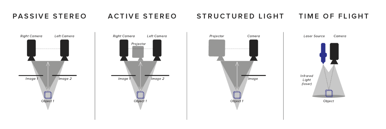
Although there are many types of depth sensor technologies (shown in Fig.1 below), they all have significant limitations.

• Time of Flight (TOF) systems suffer from motion artifacts and multi-path interference.
• Structured light is vulnerable to ambient illumination and multi-device interference.
• Passive stereo struggles in texture-less regions, where expensive global optimization techniques are required — especially in traditional non-learning based methods.

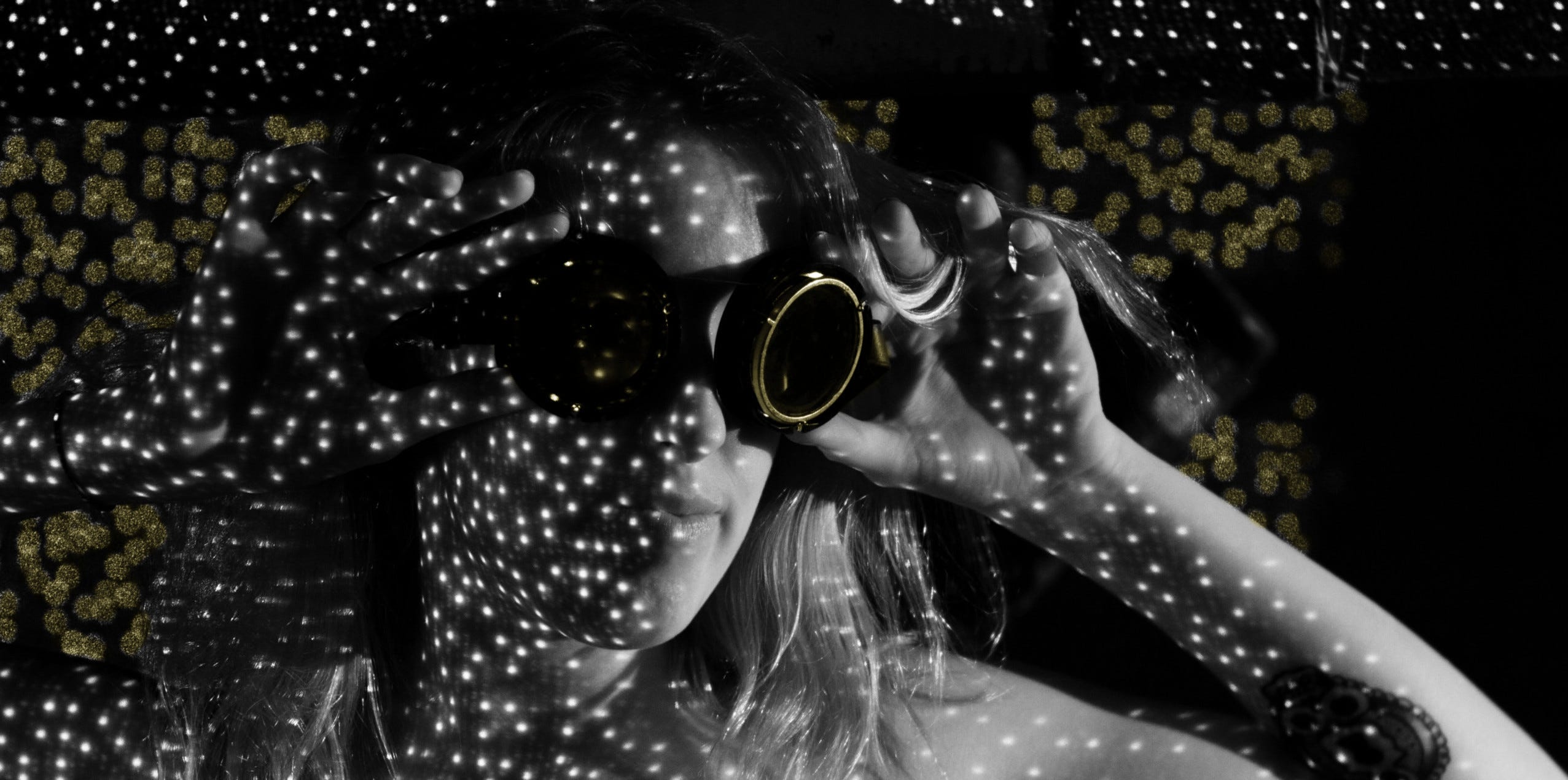
An additional depth sensor type offers a potential solution. In active stereo , an infrared stereo camera pair is used, with a pseudorandom pattern projectively texturing the scene via a patterned IR light source (Fig. 3). With a proper selection of wavelength sensing, the camera pair captures a combination of active illumination and passive light, which improves on the quality of structured light while providing a robust solution in both indoor and outdoor scenarios.

In this post, I’m going to review “ActiveStereoNet: End-to-End Self-Supervised Learning for Active Stereo Systems” , which presents an end-to-end deep learning approach for active stereo that’s trained fully self-supervised.

In this post I’ll cover two things. First, I’ll present a naive definition for active stereo. Second, an overview of “ ActiveStereoNet ”.

Table of Contents

1. Naive definition for Active Stereo

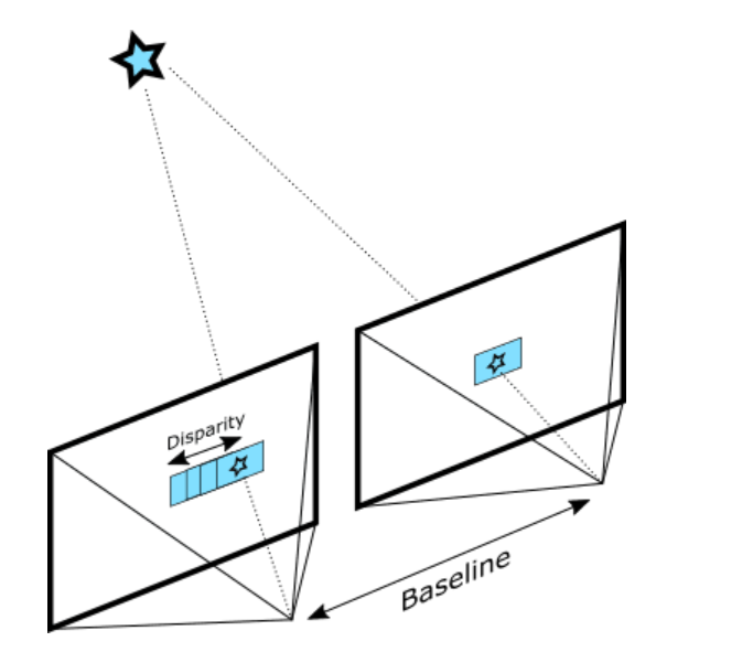
Depth from Stereo is a classic computer vision algorithm inspired by the human binocular vision system . It relies on two parallel viewports and calculates depth by estimating disparities between matching keypoints in the left and right images:

An example for the most naive implementation of this idea is the SSD (Sum of Squared Differences) block matching algorithm.

The quality of the results depends primarily on the density of visually distinguishable points (features) for the algorithm to match. Any source of texture — natural or artificial — will significantly improve the accuracy and add depth points in homogeneous areas.

That’s why it’s extremely useful to have an additional texture projector that can usually add details outside of the visible spectrum. This approach is called active stereo.

2. ActiveStereoNet: End-to-End Self-Supervised Learning for Active Stereo Systems

2.1 Intuition

Active stereo is an extension of the traditional passive stereo approach in which a texture is projected into the scene with an IR projector and cameras are augmented to perceive IR as well as visible spectra.

The general idea behind any stereo algorithm is, given a pair of rectified input images from left and right cameras, the algorithm aims to predict a disparity mapping. While most leverage a generic encoder-decoder network successful across various problems, this kind of network lacks several qualities important for stereo algorithm.

This approach does not capture any geometric intuition about the stereo matching problem. Stereo prediction is first-and-foremost a correspondence matching problem, and it’s desirable that the designed algorithm will be able to adapt without being retrained to different stereo cameras setups, e.g. varying resolution and baselines.

With this in mind, ActiveStereoNet incorporates a design that leverages the problem structure and classical approaches to tackle it.

2.2 Method & Network Structure

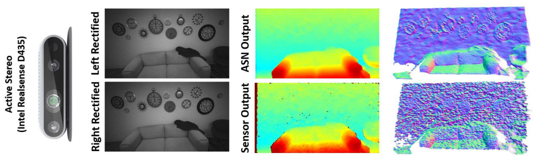
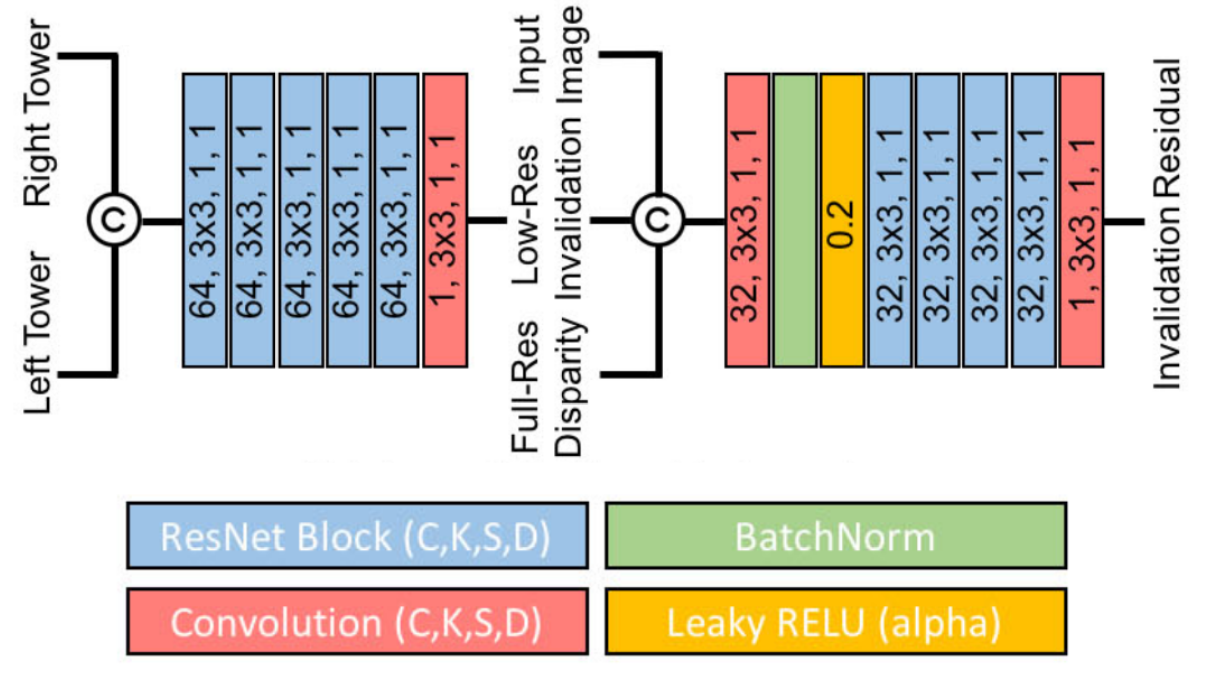
The input to ActiveStereoNet is a rectified, synchronized pair of images with active illumination (see Fig. 3), and the output is a pair of disparity maps at the original resolution.

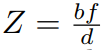
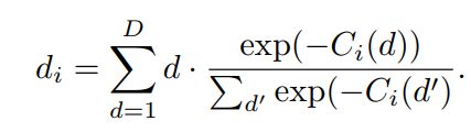
It’s worth mentioning that all experiments were performed on Intel RealSense D435 cameras that output synchronized, rectified W x H (1280 x 720) images at 30fps. With prior knowledge of the focal length f and the baseline b between the two cameras, the depth estimation problem turns into disparity d search along the epipolar line. The depth can easily be obtained via

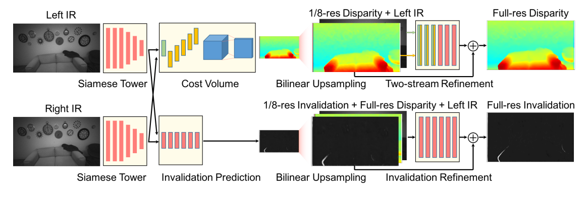
An overall network structure is shown in Fig.4 below. First, two high-resolution images go through a Siamese tower to produce a feature map in 1/8 of the input resolution. Then, a low resolution cost volume of size W/8 x H/8 x D is built, allowing for a maximum disparity of D=18 in the original image.

The cost volume produces a downsampled disparity map using a soft argmin operator . Per pixel, out of the D disparity steps calculated, the best disparity value is chosen. This results in a coarse low-resolution disparity map. This estimation is then upsampled using bi-linear interpolation to the original resolution (W× H).

A final residual refinement retrieves the high-frequency details (i.e. edges). ActiveStereoNet also simultaneously estimates an invalidation mask to remove uncertain areas in the final result.

The network’s sub-modules are described in detail in the subsections below.

2.1.1 Siamese Tower

The first step of the pipeline finds a meaningful representation of image patches that can be accurately matched in later stages. ActiveStereoNet uses a feature network with shared weights between the two input images (also known as a Siamese network).

The Siamese tower is adjusted such that it will maintain more high-frequency signals from the input image. This is accomplished by running several residual blocks on full resolution and reducing resolution later using convolution with stride. The output is a 32-dimensional feature vector at each pixel in the downsampled image of size W/8 x H/8.

2.1.2 Cost Volume

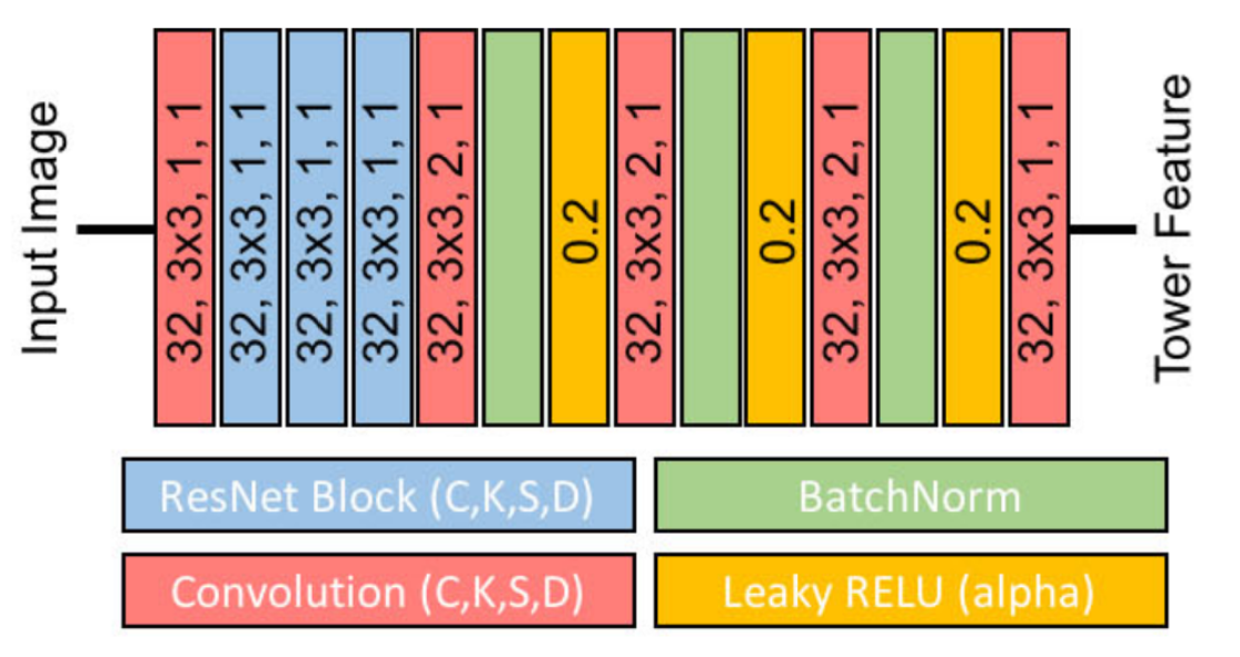
At this point, a cost-volume is formed at the coarse resolution by taking the difference between the feature vector of a pixel and the feature vectors of the matching candidates. The main idea behind this procedure is that it slides one image onto the other, finding the disparity that yields maximum correlation. In contrast to the standard approach, in ActiveStereoNet, the cost-volume is applied on the feature vector rather than on the high-resolution input images.

The animation below illustrates the procedure quite nicely. If you’re interested, you can refer to the original paper for more details on the cost-volume filter.

The input to the cost-volume is a feature vector of dimensions W/8 x H/8 x 32 that evaluates a maximum of D candidate disparities. The disparity with the minimum cost at each pixel is selected using a differentiable softmax-weighted combination of all the disparity values.

This output of size W/8 x H/8 x 1 is then upsampled using bi-linear interpolation to the original resolution W x H.

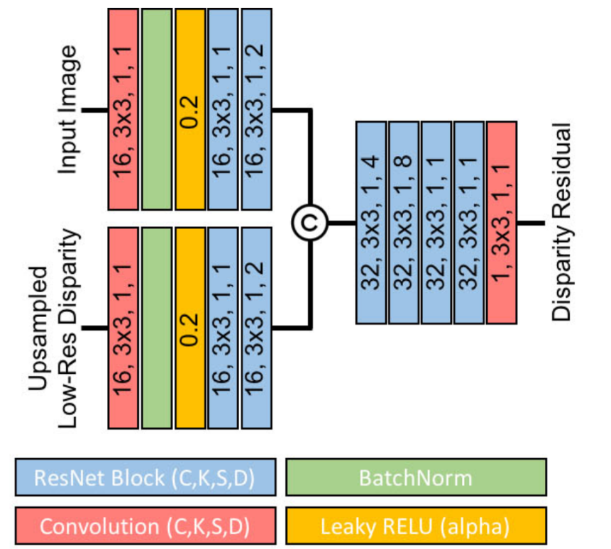
2.1.3 Residual Refinement Network

The downside of relying on coarse matching is that the resulting myopic output lacks fine details. To handle this and maintain compact design, ActiveStereoNet learns an edge-preserving refinement network.

The refinement network takes as input the disparity bi-linearly upsampled to the output size, as well as the color resized to the same dimensions.

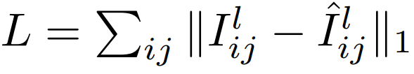
2.3 Loss

The architecture described is composed of a low-resolution disparity and a final refinement step to retrieve high-frequency details. A natural choice is to have a loss function for each of these two steps.

Due to a lack of ground truth data, ActiveStereoNet is trained in an unsupervised manner. The authors claim that while a viable choice for the training loss is the photometric error, it isn’t suitable for active cases because of a high correlation between intensity and disparity. Basically this means that brighter pixels are closer, and as pixel noise is proportional to intensity, this could lead to a network biased towards closeup scenes.

In Fig.8. below, the reconstruction error for a given disparity map using photometric loss is shown. Notice how bright pixels on the pillow exhibit high reconstruction error due to the input-dependent nature of the noise.

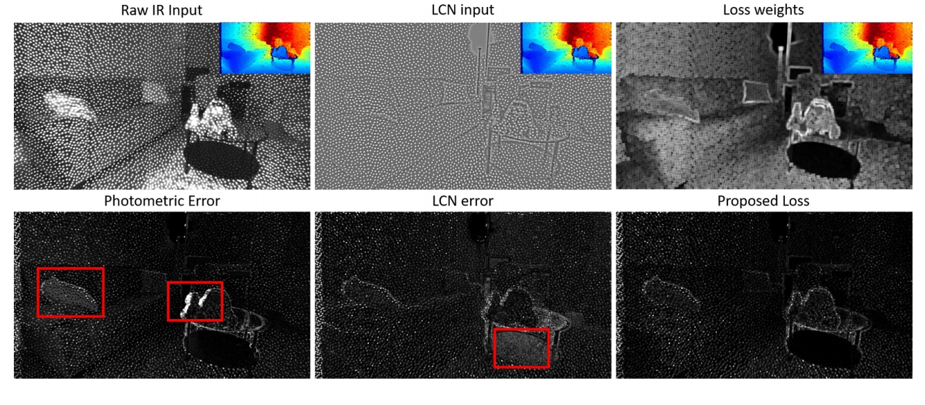
An additional issue with this loss occurs in occluded areas: indeed, when the intensity difference between background and foreground is severe, this loss will have a strong contribution in the occluded regions, forcing the network to learn to fit those areas that, however, cannot really be explained in the data.

2.3.1 Weighted Local Contrast Normalization

Here, a Local Contrast Normalization (LCN) scheme is proposed, one that not only removes the dependency between intensity and disparity, but also gives a better residual in occluded regions.

Per pixel, the local statistics are computed and used to normalize the current pixel intensity.

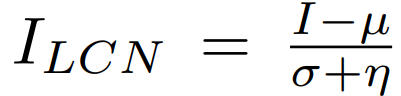
The result of this normalization is shown in Fig. 8, middle. Notice how the dependency between disparity and brightness is now removed, and moreover, the reconstruction error (Fig. 8, middle, second row) is not strongly biased towards high intensity areas or occluded regions.

The photometric loss between the original pixels on the left image I and the reconstructed left image I^ is now reformulated as follows:

Example of weights computed on the reference image are shown in Fig. 8, top right, and the final loss is shown on the bottom right. Notice how these residuals are not biased in bright areas or low-textured regions.

2.4 Invalidation Network

So far, the proposed loss doesn’t deal with occluded regions and wrong matches (i.e. textureless areas). An occluded pixel does not have any useful information in the cost volume even when brute-force search is performed.

To deal with occlusions, ActiveStereoNet uses a modified version of a traditional stereo matching method called left-right consistency check. The disparity computed from the left and right view points ( d_l & d_r respectively) are used to define a mask for a pixel p(i,j).

Those pixels with m_ij = 0 are ignored in the loss computation. In addition, to avoid having all pixels invalidated, as it is the trivial solution, a regularization is enforced. This is done by minimizing the cross-entropy loss with a constant label 1 in each valid pixel location.

As a byproduct of the invalidation network, ActiveStereoNet obtains a confidence map for the depth estimates.

4. Results

4.1 Bias and Jitter

Quantitative evaluation with state-of-the-art is shown in Fig. 10, where ActiveStereoNet achieved one order of magnitude less bias with a subpixel precision of 0.03 pixels with very low jitter.

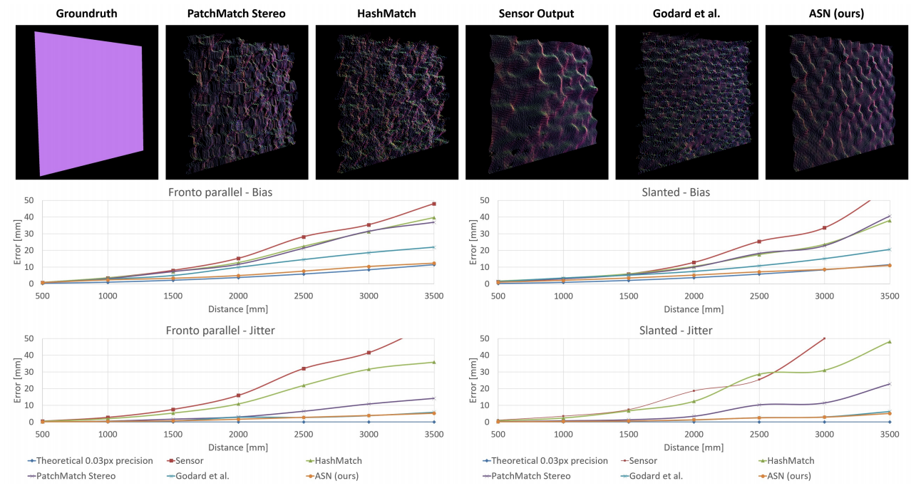
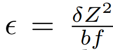
The main idea of this comparison is to test the distance error caused by the estimated disparity precision error δ. It’s known that a stereo system with baseline b, focal length f, and a subpixel disparity precision of δ, has a depth error that increases quadratically with respect to the depth Z, according to

This is accomplished by comparing the standard deviation of a “perfect” plane as “ground truth” with the standard deviation of the estimated plane. This is performed over multiple distances.

The ActiveStereoNet system performs significantly better than the other methods at all distances, and its error doesn’t increase dramatically with depth. The corresponding subpixel disparity precision of the system is 1/30th of a pixel.

In addition, to characterize the noise, the jitter was computed as the standard deviation of the depth error. Fig. 10 shows that ActiveStereoNet achieves the lowest jitter at almost every depth in comparison to other methods.

4.2 Comparisons with State-of-the-Art

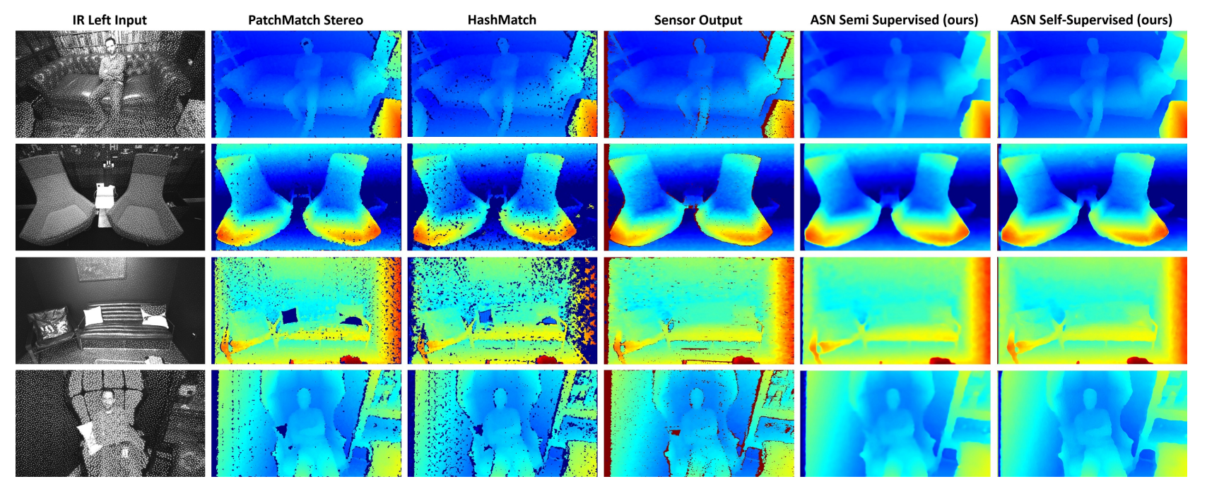
More qualitative evaluations of ASN in challenging scenes are shown in Fig. 11. As can be seen, local methods like PatchMatch stereo and HashMatch don’t handle mixed illumination with both active and passive light, and thus produce incomplete disparity images (missing pixels shown in black).

In contrast, the ASN method produces complete disparity maps and preserves sharp boundaries.