The Random Transformer

Encoder

The whole goal of the encoder is to generate a rich embedding representation of the input text. This embedding will capture semantic information about the input, and will then be passed to the decoder to generate the output text. The encoder is composed of a stack of N layers. Before we jump into the layers, we need to see how to pass the words (or tokens) into the model.

1. Embedding the text

Let’s say that we want to translate “Hello World” from English to Spanish. The first step is to turn each input token into a vector using an embedding algorithm. This is a learned encoding. Usually we use a big vector size such as 512, but let’s do 4 for our example so we can keep the maths manageable. I’ll assign some random values to each token (as mentioned, this mapping is usually learned by the model).

Hello -> [1,2,3,4]

World -> [2,3,4,5]

We can represent our input as a single matrix

E=[12342345]

2 Positional encoding

The embedding above has no information about the position of the word in the sentence, so we need to feed some positional information. The way we do this is by adding a positional encoding to the embedding. There are different choices on how to obtain these - we could use a learned embedding or a fixed vector. The original paper uses a fixed vector as they see almost no difference between the two approaches (see section 3.5 of the original paper). We’ll use a fixed vector as well. Sine and cosine functions have a wave-like pattern, and they repeat over time. By using these functions, each position in the sentence gets a unique yet consistent pattern of numbers. These are the functions they use in the paper (section 3.5):

PE(pos,2i)=sin⁡(pos100002i/dmodel)

PE(pos,2i+1)=cos⁡(pos100002i/dmodel)

The idea is to interpolate between sine and cosine for each value in the embedding (even indices will use sine, odd indices will use cosine). Let’s calculate them for our example!

For “Hello”

• i = 0 (even): PE(0,0) = sin(0 / 10000^(0 / 4)) = sin(0) = 0
• i = 1 (odd): PE(0,1) = cos(0 / 10000^(2*1 / 4)) = cos(0) = 1
• i = 2 (even): PE(0,2) = sin(0 / 10000^(2*2 / 4)) = sin(0) = 0
• i = 3 (odd): PE(0,3) = cos(0 / 10000^(2*3 / 4)) = cos(0) = 1

For “World”

• i = 0 (even): PE(1,0) = sin(1 / 10000^(0 / 4)) = sin(1 / 10000^0) = sin(1) ≈ 0.84
• i = 1 (odd): PE(1,1) = cos(1 / 10000^(2*1 / 4)) = cos(1 / 10000^0.5) ≈ cos(0.01) ≈ 0.99
• i = 2 (even): PE(1,2) = sin(1 / 10000^(2*2 / 4)) = sin(1 / 10000^1) ≈ 0
• i = 3 (odd): PE(1,3) = cos(1 / 10000^(2*3 / 4)) = cos(1 / 10000^1.5) ≈ 1

So concluding

• “Hello” -> [0, 1, 0, 1]
• “World” -> [0.84, 0.99, 0, 1]

Note that these encodings have the same dimension as the original embedding.

3. Add positional encoding and embedding

We now add the positional encoding to the embedding. This is done by adding the two vectors together.

“Hello” = [1,2,3,4] + [0, 1, 0, 1] = [1, 3, 3, 5] “World” = [2,3,4,5] + [0.84, 0.99, 0, 1] = [2.84, 3.99, 4, 6]

So our new matrix, which will be the input to the encoder, is:

E=[13352.843.9946]

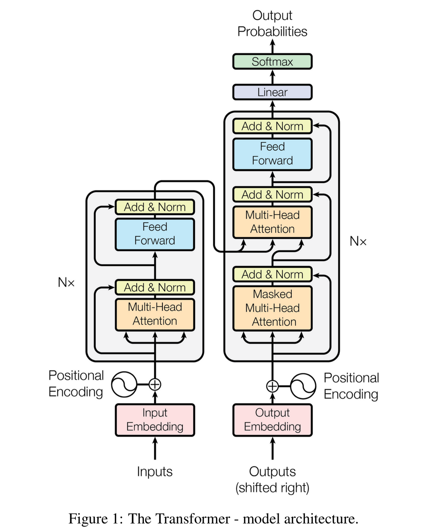
If you look at the original paper’s image, what we just did is the bottom left part of the image (the embedding + positional encoding).

Transformer model from the original “attention is all you need” paper

4. Self-attention

4.1 Matrices Definition

We’ll now introduce the concept of multi-head attention. Attention is a mechanism that allows the model to focus on certain parts of the input. Multi-head attention is a way to allow the model to jointly attend to information from different representation subspaces. This is done by using multiple attention heads. Each attention head will have its own K, V, and Q matrices.

Let’s use 2 attention heads for our example. We’ll use random values for these matrices. Each matrix will be a 4x3 matrix. With this, each matrix will transform the 4-dimensional embeddings into 3-dimensional keys, values, and queries. This reduces the dimensionality for attention mechanism, which helps in managing the computational complexity. Note that using a too small attention size will hurt the performance of the model. Let’s use the following values (just random values):

For the first head

WK1=[101010101010],WV1=[011100101010],WQ1=[000110001110]

For the second head

WK2=[011101101010],WV2=[100011001100],WQ2=[101010100011]

4.2 Keys, queries, and values calculation

We now need to multiply our input embeddings with the weight matrices to obtain the keys, queries, and values.

Key calculation

E×WK1=[13352.843.9946][101010101010]=[(1×1)+(3×0)+(3×1)+(5×0)(1×0)+(3×1)+(3×0)+(5×1)(1×1)+(3×0)+(3×1)+(5×0)(2.84×1)+(3.99×0)+(4×1)+(6×0)(2.84×0)+(4×1)+(4×0)+(6×1)(2.84×1)+(4×0)+(4×1)+(6×0)]=[4846.849.996.84]

Ok, I actually do not want to do the math by hand for all of these - it gets a bit repetitive plus it breaks the site. So let’s cheat and use NumPy to do the calculations for us.

We first define the matrices

import numpy as np

WK1 = np.array([[1, 0, 1], [0, 1, 0], [1, 0, 1], [0, 1, 0]])
WV1 = np.array([[0, 1, 1], [1, 0, 0], [1, 0, 1], [0, 1, 0]])
WQ1 = np.array([[0, 0, 0], [1, 1, 0], [0, 0, 1], [1, 0, 0]])

WK2 = np.array([[0, 1, 1], [1, 0, 1], [1, 1, 0], [0, 1, 0]])
WV2 = np.array([[1, 0, 0], [0, 1, 1], [0, 0, 1], [1, 0, 0]])
WQ2 = np.array([[1, 0, 1], [0, 1, 0], [1, 0, 0], [0, 1, 1]])

And let’s confirm that I didn’t make any mistakes in the calculations above.

embedding = np.array([[1, 3, 3, 5], [2.84, 3.99, 4, 6]])
K1 = embedding @ WK1
K1

array([[4.  , 8.  , 4.  ],
       [6.84, 9.99, 6.84]])

Phew! Let’s now get the values and queries

Value calculations

V1 = embedding @ WV1
V1

array([[6.  , 6.  , 4.  ],
       [7.99, 8.84, 6.84]])

Query calculations

Q1 = embedding @ WQ1
Q1

array([[8.  , 3.  , 3.  ],
       [9.99, 3.99, 4.  ]])

Let’s skip the second head for now and focus on the first head final score. We’ll come back to the second head later.

4.3 Attention calculation

Calculating the attention score requires a couple of steps:

1. Calculate the dot product of the query with each key
2. Divide the result by the square root of the dimension of the key vector
3. Apply a softmax function to obtain the attention weights
4. Multiply each value vector by the attention weights

4.3.1 Dot product of query with each key

The score for “Hello” requires calculating the dot product of q1 with each key vector (k1 and k2)

q1⋅k1=[833]⋅[484]=8⋅4+3⋅8+3⋅4=68

In matrix world, that would be Q1 multiplied by the transpose of K1

Q1×K1⊤=[8339.993.994]×[46.8489.9946.84]=[8⋅4+3⋅8+3⋅48⋅6.84+3⋅9.99+3⋅6.849.99⋅4+3.99⋅8+4⋅49.99⋅6.84+3.99⋅9.99+4⋅6.84]=[68105.2187.88135.5517]

I’m prone to do mistakes, so let’s confirm with Python once again

scores1 = Q1 @ K1.T
scores1

array([[ 68.    , 105.21  ],
       [ 87.88  , 135.5517]])

4.3.2 Divide by square root of dimension of key vector

We then divide the scores by the square root of the dimension (d) of the keys (3 in this case, but 64 in the original paper). Why? For large values of d, the dot product grows too large (we’re adding the multiplication of a bunch of numbers, after all, leading to high values). And large values are bad! We’ll discuss soon more about this.

scores1 = scores1 / np.sqrt(3)
scores1

array([[39.2598183 , 60.74302182],
       [50.73754166, 78.26081048]])

4.3.3 Apply softmax function

We then softmax to normalize so they are all positive and add up to 1.

def softmax(x):
    return np.exp(x) / np.sum(np.exp(x), axis=1, keepdims=True)


scores1 = softmax(scores1)
scores1

array([[4.67695573e-10, 1.00000000e+00],
       [1.11377182e-12, 1.00000000e+00]])

4.3.4 Multiply value matrix by attention weights

We then multiply times the value matrix

attention1 = scores1 @ V1
attention1

array([[7.99, 8.84, 6.84],
       [7.99, 8.84, 6.84]])

Let’s combine 4.3.1, 4.3.2, 4.3.3, and 4.3.4 into a single formula using matrices (this is from section 3.2.1 of the original paper):

Attention(Q,K,V)=softmax(QK⊤d)V

Yes, that’s it! All the math we just did can easily be encapsulated in the attention formula above! Let’s now translate this to code!

def attention(x, WQ, WK, WV):
    K = x @ WK
    V = x @ WV
    Q = x @ WQ

    scores = Q @ K.T
    scores = scores / np.sqrt(3)
    scores = softmax(scores)
    scores = scores @ V
    return scores

attention(embedding, WQ1, WK1, WV1)

array([[7.99, 8.84, 6.84],
       [7.99, 8.84, 6.84]])

We confirm we got same values as above. Let’s chear and use this to obtain the attention scores the second attention head:

attention2 = attention(embedding, WQ2, WK2, WV2)
attention2

array([[8.84, 3.99, 7.99],
       [8.84, 3.99, 7.99]])

If you’re wondering how come the attention is the same for the two embeddings, it’s because the softmax is taking our scores to 0 and 1. See this:

softmax(((embedding @ WQ2) @ (embedding @ WK2).T) / np.sqrt(3))

array([[1.10613872e-14, 1.00000000e+00],
       [4.95934510e-20, 1.00000000e+00]])

This is due to bad initialization of the matrices and small vector sizes. Large differences in the scores before applying softmax will just be amplified with softmax, leading to one value being close to 1 and others close to 0. In practice, our initial embedding matrices’ values were maybe too high, leading to high values for the keys, values, and queries, which just grew larger as we multiplied them.

Remember when we were dividing by the square root of the dimension of the keys? This is why we do that. If we don’t do that, the values of the dot product will be too large, leading to large values after the softmax. In this case, though, it seems it wasn’t enough given our small values! As a short-term hack, we can scale down the values by a larger amount than the square root of 3. Let’s redefine the attention function but scaling down by 30. This is not a good long-term solution, but it will help us get different values for the attention scores. We’ll get back to a better solution later.

def attention(x, WQ, WK, WV):
    K = x @ WK
    V = x @ WV
    Q = x @ WQ

    scores = Q @ K.T
    scores = scores / 30  # we just changed this
    scores = softmax(scores)
    scores = scores @ V
    return scores

attention1 = attention(embedding, WQ1, WK1, WV1)
attention1

array([[7.54348784, 8.20276657, 6.20276657],
       [7.65266185, 8.35857269, 6.35857269]])

attention2 = attention(embedding, WQ2, WK2, WV2)
attention2

array([[8.45589591, 3.85610456, 7.72085664],
       [8.63740591, 3.91937741, 7.84804146]])

4.3.5 Heads’ attention output

The next layer of the encoder will expect a single matrix, not two. The first step will be to concatenate the two heads’ outputs (section 3.2.2 of the original paper)

attentions = np.concatenate([attention1, attention2], axis=1)
attentions

array([[7.54348784, 8.20276657, 6.20276657, 8.45589591, 3.85610456,
        7.72085664],
       [7.65266185, 8.35857269, 6.35857269, 8.63740591, 3.91937741,
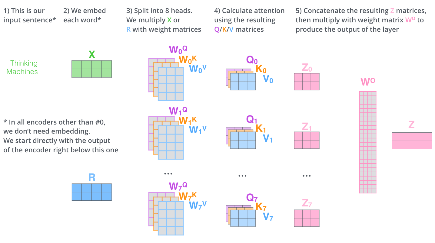
        7.84804146]])

We finally multiply this concatenated matrix by a weight matrix to obtain the final output of the attention layer. This weight matrix is also learned! The dimension of the matrix ensures we go back to the same dimension as the embedding (4 in our case).

# Just some random values
W = np.array(
    [
        [0.79445237, 0.1081456, 0.27411536, 0.78394531],
        [0.29081936, -0.36187258, -0.32312791, -0.48530339],
        [-0.36702934, -0.76471963, -0.88058366, -1.73713022],
        [-0.02305587, -0.64315981, -0.68306653, -1.25393866],
        [0.29077448, -0.04121674, 0.01509932, 0.13149906],
        [0.57451867, -0.08895355, 0.02190485, 0.24535932],
    ]
)
Z = attentions @ W
Z

array([[ 11.46394285, -13.18016471, -11.59340253, -17.04387829],
       [ 11.62608573, -13.47454936, -11.87126395, -17.4926367 ]])

The image from The Ilustrated Transformer encapsulates all of this in a single image

5. Feed-forward layer

5.1 Basic feed-forward layer

After the self-attention layer, the encoder has a feed-forward neural network (FFN). This is a simple network with two linear transformations and a ReLU activation in between. The Illustrated Transformer blog post does not dive into it, so let me briefly explain a bit more. The goal of the FFN is to process and transformer the representation produced by the attention mechanism. The flow is usually as follows (see section 3.3 of the original paper):

1. First linear layer: this usually expands the dimensionality of the input. For example, if the input dimension is 512, the output dimension might be 2048. This is done to allow the model to learn more complex functions. In our simple of example with dimension of 4, we’ll expand to 8.
2. ReLU activation: This is a non-linear activation function. It’s a simple function that returns 0 if the input is negative, and the input if it’s positive. This allows the model to learn non-linear functions. The math is as follows:

ReLU(x)=max(0,x)

1. Second linear layer: This is the opposite of the first linear layer. It reduces the dimensionality back to the original dimension. In our example, we’ll reduce from 8 to 4.

We can represent all of this as follows

FFN(x)=ReLU(xW1+b1)W2+b2

Just as a reminder, the input for this layer is the Z we calculated in the self-attention above. Here are the values as a reminder

Z=[11.46394281−13.18016469−11.59340253−17.0438783311.62608569−13.47454934−11.87126395−17.49263674]

Let’s now define some random values for the weight matrices and bias vectors. I’ll do it with code, but you can do it by hand if you feel patient!

W1 = np.random.randn(4, 8)
W2 = np.random.randn(8, 4)
b1 = np.random.randn(8)
b2 = np.random.randn(4)

And now let’s write the forward pass function

def relu(x):
    return np.maximum(0, x)

def feed_forward(Z, W1, b1, W2, b2):
    return relu(Z.dot(W1) + b1).dot(W2) + b2

output_encoder = feed_forward(Z, W1, b1, W2, b2)
output_encoder

array([[ -3.24115016,  -9.7901049 , -29.42555675, -19.93135286],
       [ -3.40199463,  -9.87245924, -30.05715408, -20.05271018]])

5.2 Encapsulating everything: The Random Encoder

Let’s now write some code to have the multi-head attention and the feed-forward, all together in the encoder block.

d_embedding = 4
d_key = d_value = d_query = 3
d_feed_forward = 8
n_attention_heads = 2

def attention(x, WQ, WK, WV):
    K = x @ WK
    V = x @ WV
    Q = x @ WQ

    scores = Q @ K.T
    scores = scores / np.sqrt(d_key)
    scores = softmax(scores)
    scores = scores @ V
    return scores

def multi_head_attention(x, WQs, WKs, WVs):
    attentions = np.concatenate(
        [attention(x, WQ, WK, WV) for WQ, WK, WV in zip(WQs, WKs, WVs)], axis=1
    )
    W = np.random.randn(n_attention_heads * d_value, d_embedding)
    return attentions @ W

def feed_forward(Z, W1, b1, W2, b2):
    return relu(Z.dot(W1) + b1).dot(W2) + b2

def encoder_block(x, WQs, WKs, WVs, W1, b1, W2, b2):
    Z = multi_head_attention(x, WQs, WKs, WVs)
    Z = feed_forward(Z, W1, b1, W2, b2)
    return Z

def random_encoder_block(x):
    WQs = [
        np.random.randn(d_embedding, d_query) for _ in range(n_attention_heads)
    ]
    WKs = [
        np.random.randn(d_embedding, d_key) for _ in range(n_attention_heads)
    ]
    WVs = [
        np.random.randn(d_embedding, d_value) for _ in range(n_attention_heads)
    ]
    W1 = np.random.randn(d_embedding, d_feed_forward)
    b1 = np.random.randn(d_feed_forward)
    W2 = np.random.randn(d_feed_forward, d_embedding)
    b2 = np.random.randn(d_embedding)
    return encoder_block(x, WQs, WKs, WVs, W1, b1, W2, b2)

Recall that our input is the matrix E which has the positional encoding and the embedding.

embedding

array([[1.  , 3.  , 3.  , 5.  ],
       [2.84, 3.99, 4.  , 6.  ]])

Let’s now pass this to our random_encoder_block function

random_encoder_block(embedding)

array([[ -71.76537515, -131.43316885,   13.2938131 ,   -4.26831998],
       [ -72.04253781, -131.84091347,   13.3385937 ,   -4.32872015]])

Nice! This was just one encoder block. The original paper uses 6 encoders. The output of one encoder goes to the next, and so on:

def encoder(x, n=6):
    for _ in range(n):
        x = random_encoder_block(x)
    return x


encoder(embedding)

/tmp/ipykernel_11906/1045810361.py:2: RuntimeWarning: overflow encountered in exp
  return np.exp(x)/np.sum(np.exp(x),axis=1, keepdims=True)
/tmp/ipykernel_11906/1045810361.py:2: RuntimeWarning: invalid value encountered in divide
  return np.exp(x)/np.sum(np.exp(x),axis=1, keepdims=True)

array([[nan, nan, nan, nan],
       [nan, nan, nan, nan]])

5.3 Residual and Layer Normalization

Uh oh! We’re getting NaNs! It seems our values are too high, and when being passed to the next encoder, they end up being too high and exploding! This is called gradient explosion. Without any kind of normalization, small changes in the input of early layers end up being amplified in later layers. This is a common problem in deep neural networks. There are two common techniques to mitigate this problem: residual connections and layer normalization (section 3.1 of the paper, barely mentioned).

• Residual connections: Residual connections are simply adding the input of the layer to it output. For example, we add the initial embedding to the output of the attention. Residual connections mitigate the vanishing gradient problem. The intuition is that if the gradient is too small, we can just add the input to the output and the gradient will be larger. The math is very simple:

Residual(x)=x+Layer(x)

That’s it! We’ll do this to the output of the attention and the output of the feed-forward layer.

• Layer normalization Layer normalization is a technique to normalize the inputs of a layer. It normalizes across the embedding dimension. The intuition is that we want to normalize the inputs of a layer so that they have a mean of 0 and a standard deviation of 1. This helps with the gradient flow. The math does not look so simple at a first glance.

LayerNorm(x)=x−μσ2+ϵ×γ+β

Let’s explain each parameter:

• μ is the mean of the embedding
• σ is the standard deviation of the embedding
• ϵ is a small number to avoid division by zero. In case the standard deviation is 0, this small epsilon saves the day!
• γ and β are learned parameters that control scaling and shifting steps.

Unlike batch normalization (no worries if you don’t know what it is), layer normalization normalizes across the embedding dimension - that means that each embedding will not be affected by other samples in the batch. The intuition is that we want to normalize the inputs of a layer so that they have a mean of 0 and a standard deviation of 1.

Why do we add the learnable parameters γ and β? The reason is that we don’t want to lose the representational power of the layer. If we just normalize the inputs, we might lose some information. By adding the learnable parameters, we can learn to scale and shift the normalized values.

Combining the equations, the equation for the whole encoder could look like this

Z(x)=LayerNorm(x+Attention(x))

FFN(x)=ReLU(xW1+b1)W2+b2

Encoder(x)=LayerNorm(Z(x)+FFN(Z(x)+x))

Let’s try with our example! Let’s go with E and Z values from before

E+Attention(E)=[1.03.03.05.02.843.994.06.0]+[11.46394281−13.18016469−11.59340253−17.0438783311.62608569−13.47454934−11.87126395−17.49263674]=[12.46394281−10.18016469−8.59340253−12.0438783314.46608569−9.48454934−7.87126395−11.49263674]

Let’s now calculate the layer normalization, we can divide it into three steps:

1. Compute mean and variance for each embedding.
2. Normalize by substracting the mean of its row and dividing by the square root of its row variance (plus a small number to avoid division by zero).
3. Scale and shift by multiplying by gamma and adding beta.

5.3.1 Mean and variance

For the first embedding

μ1=12.46394281−10.18016469−8.59340253−12.043878334=−4.58837568σ2=∑(xi−μ)2N=(12.46394281−(−4.588375685))2+…+(−12.04387833−(−4.588375685))24=393.674430050134=98.418607512533σ=98.418607512533=9.9206152789297

We can do the same for the second embedding. We’ll skip the calculations but you get the hang of it.

μ2=−3.59559109σ2=10.50653018

Let’s confirm with Python

(embedding + Z).mean(axis=-1, keepdims=True)

array([[-4.58837567],
       [-3.59559107]])

(embedding + Z).std(axis=-1, keepdims=True)

array([[ 9.92061529],
       [10.50653019]])

Amazing! Let’s now normalize

5.3.2 Normalize

For normalization, for each value in the embedding, we subsctract the mean and divide by the standard deviation. Epsilon is a very small value, such as 0.00001. We’ll assume γ=1 and β=0, it simplifies things.

normalized1=12.46394281−(−4.58837568)98.418607512533+ϵ=17.052318499.9206152789297=1.718normalized2=−10.18016469−(−4.58837568)98.418607512533+ϵ=−5.591789019.9206152789297=−0.564normalized3=−8.59340253−(−4.58837568)98.418607512533+ϵ=−4.005026859.9206152789297=−0.404normalized4=−12.04387833−(−4.58837568)98.418607512533+ϵ=−7.455502659.9206152789297=−0.752

We’ll skip the calculations by hand for the second embedding. Let’s confirm with code! Let’s re-define our encoder_block function with this change

def layer_norm(x, epsilon=1e-6):
    mean = x.mean(axis=-1, keepdims=True)
    std = x.std(axis=-1, keepdims=True)
    return (x - mean) / (std + epsilon)

def encoder_block(x, WQs, WKs, WVs, W1, b1, W2, b2):
    Z = multi_head_attention(x, WQs, WKs, WVs)
    Z = layer_norm(Z + x)

    output = feed_forward(Z, W1, b1, W2, b2)
    return layer_norm(output + Z)

layer_norm(Z + embedding)

array([[ 1.71887693, -0.56365339, -0.40370747, -0.75151608],
       [ 1.71909039, -0.56050453, -0.40695381, -0.75163205]])

It works! Let’s retry to pass the embedding through the six encoders.

def encoder(x, n=6):
    for _ in range(n):
        x = random_encoder_block(x)
    return x


encoder(embedding)

array([[-0.335849  , -1.44504571,  1.21698183,  0.56391289],
       [-0.33583947, -1.44504861,  1.21698606,  0.56390202]])

Amazing! These values make sense and we don’t get NaNs! The idea of the stack of encoders is that they output a continuous representation, z, that captures the meaning of the input sequence. This representation is then passed to the decoder, which will genrate an output sequence of symbols, one element at a time.

Before diving into the decoder, here’s an image from Jay’s amazing blog post:

Encoder and decoder

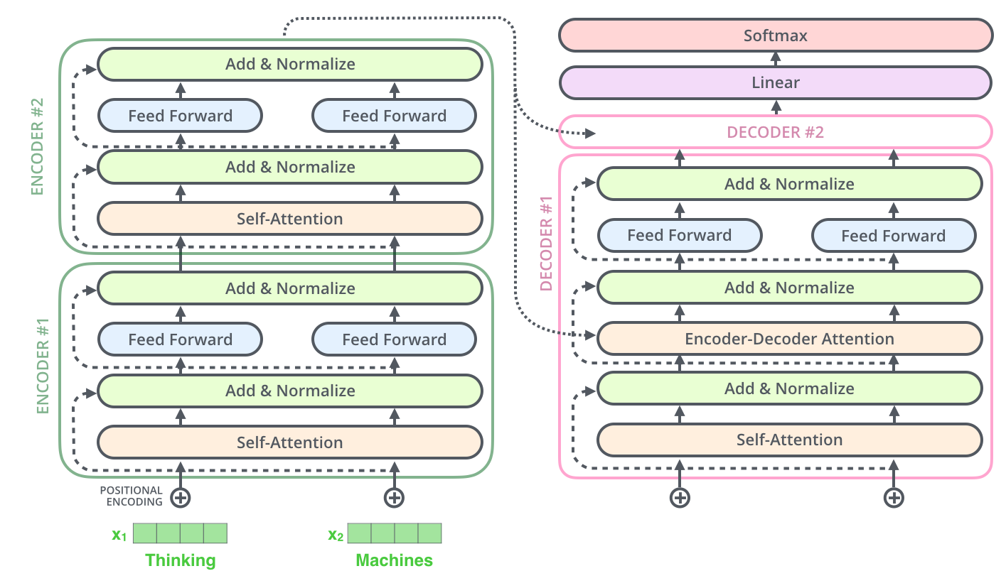
You should be able to explain each component at the left side! Quite impressive, right? Let’s now move to the decoder.