Moiré effect in displays: a tutorial

Introduction

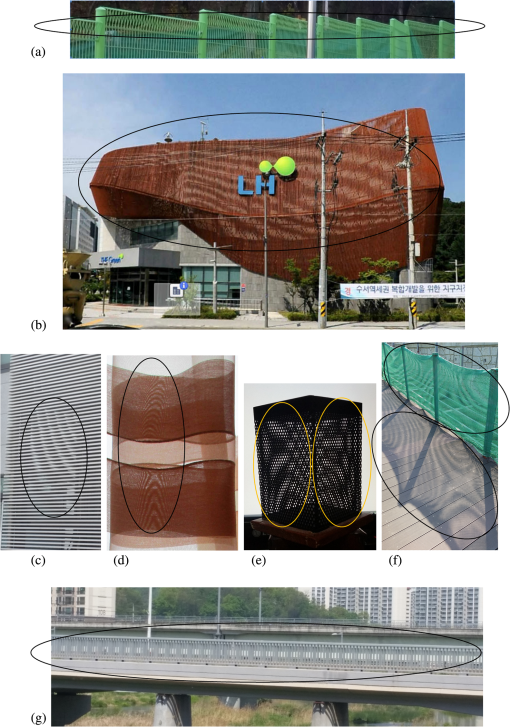
The moiré effect is a physical phenomenon of linear optics. The moiré patterns appear as a result of an interaction between transparent layers of a repeated structure1 when superposed layers are viewed through. Several examples of the moiré effect are shown in Fig. 1 (a bridge, a facade of a building, an air conditioner grid, a textile curtain, etc.).

Fig. 1Download

Moiré patterns around us (a) fence, (b) building, (c) air conditioner grid of a building (d) curtain, (e) pen holder, (f) mesh and its shadow, and (g) bridge.

The visual appearance of the moiré patterns depends on characteristics of gratings and on the location of the observer.2 In the case of two gratings, the patterns look like an added series of repeated stripes, which could look bright, vivid, and sometimes even unpredictable.

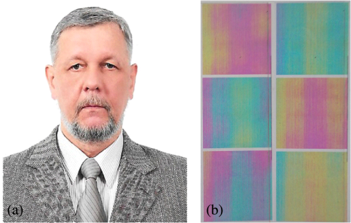
The moiré effect is not unknown in the literature. A general description of the moiré effect can be found in several books (Refs. 1–3), which also include many useful examples. A perfectly illustrated book, Ref. 4 is full of excellent moiré images. There are also research papers, specifically Refs. 56.7.8.9.–10, which describe various aspects of the moiré effect. Examples of the moiré effect in digital devices are shown in Fig. 2.

Fig. 2Download

Moiré patterns in the digital world (a) scanned image and (b) 3-D displays.

In gratings of similar layouts, the moiré patterns reproduce the structure of the gratings as in the moiré magnifier,11 see Fig. 3. This figure also shows that with all other conditions equal, the period of the moiré patterns is the same in gratings of different geometric layouts.

Fig. 3Download

Same period of moiré patterns in (a) square and (b) hexagonal grids of identical periods.

Generally speaking, visual displays can be either dynamic or static. The dynamic displays are CRT TV, LCD, and OLED. The examples of static displays are a printed picture or photograph, poster, and postcard. In visual displays, the moiré effect may create an unwanted and sometimes unexpected image of bands (as in Fig. 1) or patterns (as in Fig. 3). Such additional visual background decreases the contrast on the display screen and consequently reduces the image quality; therefore in imaging and displays, the moiré effect is an undesirable adverse visual effect.12,13 The elimination or the reduction of the moiré patterns in displays is an important issue of improvement in the visual quality. The necessity of the minimization of the moiré patterns in three-dimensional (3-D) displays was first stated14 in the early 2000s. This is especially important for autostereoscopic 3-D displays,15–23 where the moiré effect may often occur due to their typical design.

The moiré effect was observed not only under visible light but also under rays and beams of different nature, for instance, in electron beams,23 infrared light,24 and x-rays,25 as well as at the nanoscale in graphene layers.26

Finding characteristics of patterns based on the layouts of the layers is a direct problem.27–31 An inverse problem is to find the position (shape) of another grating based on the observed moiré patterns when positions of an observer and of one grating are known together with the parameters of the grating; this is a topic of the 3-D shape measurement.2,32–37

In contrast, it appears to be possible to arrange the moiré patterns so the resulting pattern would carry useful informational content (including 3-D). The first solution of this previously unknown moiré problem was proposed in Ref. 38 and implemented in Ref. 39. Also, the moiré effect can be used for other purposes, such as the moiré interferometry,40–42 the moiré deflectometry,43 the optical alignment,44,45 the visual security (cryptography),46,47 and many other applications.

That is to say, this is a twofold moiré problem that on the one hand, deals with minimization of the moiré effect to improve the image quality;48 and on the other hand, with its maximization to measure distances,49,50 as well as to display meaningful images38 in 3-D displays based entirely on the moiré effect as the main physical principle, or to improve security.51–53 An image in a 3-D moiré display is shown in Fig. 4. In each application example mentioned in this paragraph, the understanding of the behavior of the moiré patterns is needed.

Fig. 4Download

Image in a moiré display.

There are many approaches to investigate the moiré effect. In some cases, solutions can be found from direct analytical considerations. The indicial method can be used to find locations of the characteristic points (minima or maxima) of the patterns. The indicial and direct approaches require simplification, such as a simplified structure, small angles, smooth functions (nearly sinusoidal), etc.

Dealing with spectra represents a generalized approach.54–56 Using spectral trajectories,57 the behavior of the patterns can be estimated geometrically. As the equations of the trajectories are derived from the geometric characteristics of the gratings, the estimation can be made without calculations of spectra. This makes the spectral trajectories suitable for an interactive computer simulation.

The tutorial is based on the authors’ knowledge and comprehension of the moiré phenomenon and experience in investigating it for a decade. It includes several methods to find characteristics of the moiré patterns in various situations that are presented.

After sections, we provide exercises. We hope that the exercises can make readers to think deeply, and this way to improve their understanding of the considered topics. Implied is a self-check as, for example, the same result obtained by an independent method. This is probably one of the best methods of verification. Nevertheless, whenever readers would send their solutions to the authors, the readers’ notes and comments will be considered and replied to with the greatest pleasure.

The tutorial is arranged as follows: Secs. 2–5 deal with the moiré effect directly, in the spatial domain, whereas Secs. 6–8 deal with spectra (the spectral domain). Namely, in Sec. 2, we explain the indicial equation method. In Secs. 3 and 4, we describe the plain coplanar and noncoplanar sinusoidal gratings. Section 5 gives an example of the moiré effect in a 3-D object, a cylinder. Then, Secs. 6 and 7 present such fundamental issues as the wave vector of the moiré patterns in terms of the vector sum and the basics of two-dimensional (2-D) Fourier transform. Section 8 describes the spectral trajectories. After discussion about the visual effects in displaced or rotated plane gratings in Sec. 9, a conclusion finalizes the tutorial.

Indicial Equation

The indicial equation is an analytical method to calculate the characteristic locations of fringes, implying that the locations of the minima/maxima of gratings are known. In this approach, a line grating is modeled by a series of thin lines (a sketch of a family of lines), i.e., some kind of a wireframe of the maxima (or minima) only, with the intensity profile ignored. The lines of the moiré bands connect the intersections of these families of lines of gratings. As soon as the equations of these intersections can be calculated based on the given equations of the families, technically the equations of the moiré bands can be found as analytical expressions.

As an easy example, consider two families of the equidistant parallel lines in the xyxy-plane: the horizontal lines with period T1T1 and the slanted lines with period T2T2 (rotated at the angle αα). The sketch lines of the gratings are shown by solid lines in Fig. 5; the moiré patterns comprise the third family of lines with the period TmTm at the angle θθ (shown by dotted lines connecting the intersections in a shortest way). These spots or relatively low visual densities are visually connected as brighter spaces between darker areas, and the moiré patterns appear.

Fig. 5Download

Sketch of the indices.

The periods of bright and dark lines are identical. Without loss of generality, consider the maxima. The equations of two families are

Excluding mm and nn from Eqs. (1)–(3), we obtain the equation of the qq’th intersection, i.e., the qq’th moiré line

This equation represents the family of the parallel lines of lower spatial frequency (whose period is longer than the period of either grating). From the equation of the straight line, Eq. (4) can be rewritten in the normal form

In the case of the identical gratings (T1=T2T1=T2), Eqs. (6) and (7) are simplified. The angle becomes

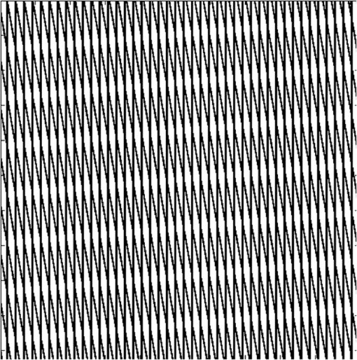
Equations (6) and (7) correspond to Eq. (2.9) from Ref. 1 with θ1=0θ1=0, whereas Eqs. (8) and (9) correspond to Eq. (2.10) there. A visual illustration of the moiré effect in the identical gratings is shown in Fig. 6 (α=5degα=5deg).

Fig. 6Download

Moiré patterns in overlapped gratings.

Sinusoidal Coplanar Gratings

The profile of the gratings also can be taken into account. For example, the analytical expressions of the moiré bands can be obtained for the sinusoidal gratings. The moiré patterns are the patterns of a longer period. The estimation of their visual appearance is based on the wave numbers.

Two Line Gratings

An interaction between the gratings can be modeled mathematically by the multiplication of transparency functions of the gratings. For instance, a one-dimensional (1-D) sinusoidal line grating (whose intensity profile along certain direction is a sinusoidal function) can be described by its transparency function t=(1+cosk⋅x)/2t=(1+cosk·x)/2, where kk is the wave vector (inversely proportional to the period), and xx is the coordinate axis. A sinusoidal grating is shown in Fig. 7(a).

Fig. 7Download

(a) Sinusoidal 1-D grating and (b) sinusoidal 2-D grid.

A result of the interaction between two gratings Fig. 7(a) can be written as

Eq. (10)

t12=t1t2=12[1+cos(k1⋅x)]⋅12[1+cos(k2⋅x)]=14[1+cos(k1⋅x)+cos(k2⋅x)+cos(k1⋅x)cos(k2⋅x)]=14{1+cos(k1⋅x)+cos(k2⋅x)+12cos[(k1+k2)⋅x]+12cos[(k1−k2)⋅x]},t12=t1t2=12[1+cos(k1·x)]·12[1+cos(k2·x)]=14[1+cos(k1·x)+cos(k2·x)+cos(k1·x)cos(k2·x)]=14{1+cos(k1·x)+cos(k2·x)+12cos[(k1+k2)·x]+12cos[(k1−k2)·x]},

where k1k1 and k2k2 are the wave vectors of the gratings; the expression k⋅xk·x means the dot product of the vectors kk and xx.

For the moiré effect, we need the smallest wave number. In Eq. (10), the first term is the constant bias (a “DC” term), the second and third terms are the gratings themselves, whereas the fourth and fifth terms represent combinational spatial frequencies (sum and difference). In Eq. (10), the term with the smallest wave number (and with the lowest spatial frequency) is the fourth term proportional to cos[(k1−k2)⋅x]cos[(k1−k2)·x].

Square Grid + Line Grating

Superimposed gratings model a typical structure of many displays. A square grid can be thought as a pair of overlapped orthogonal gratings, whereas the barrier (or lenticular) plate can be modeled by a line grating. Accordingly, for two superposed rectangular gratings, we need two such pairs, four gratings total. For the square grid superposed with the line grating, we need three gratings. Examples of the grating and the grid are shown in Fig. 7.

The transparency function of overlapped gratings obtained by the multiplication is

Eq. (11)

t123=t1t2t3=116[1+cos(k1x⋅x1)][1+cos(k1y⋅y1)][1+cos(k2x⋅x2)].t123=t1t2t3=116[1+cos(k1x·x1)][1+cos(k1y·y1)]⁢[1+cos(k2x·x2)].

The vector relationship Eq. (11) can be rewritten in a scalar form. For that purpose, the dot products in Eq. (11) can be rewritten as follows:

Eq. (12)

k1x⋅x1=ρk(1,0)⋅(x,y)=ρkxk1y⋅y1=ρk(0,1)⋅(x,y)=ρkyk2x⋅x2=k(cosα,sinα)⋅(x,y)=k(xcosα+ysinα),k1x·x1=ρk(1,0)·(x,y)=ρkxk1y·y1=ρk(0,1)·(x,y)=ρkyk2x·x2=k(cosα,sinα)·(x,y)=k(xcosα+ysinα),

where kk is the wave number of the first grating, αα is the angle between the wave vectors of the gratings, and

Eq. (13)

ρ=k1/k2,ρ=k1/k2,

is the ratio of wave numbers which are the moduli of the corresponding wave vectors as follows, k1=|k1|,k2=|k2|k1=|k1|,k2=|k2|. Substituting Eq. (12) into Eq. (11), we have

Eq. (14)

t123=t1t2t3=116(1+cosρkx)(1+cosρky){1+cos[k(xcosα+ysinα)]}=116(1+cosρkx+cosρky+cosρkxcosρky){1+cos[k(xcosα+ysinα)]}=116[1+cosρkx+cosρky+12cosρ(kx−ky)+12cosρ(kx+ky)]{1+cos[k(xcosα+ysinα)]}.t123=t1t2t3=116(1+cosρkx)(1+cosρky)⁢{1+cos[k(xcosα+ysinα)]}=116(1+cosρkx+cosρky+cosρkxcosρky)⁢{1+cos[k(xcosα+ysinα)]}=116[1+cosρkx+cosρky+12cosρ(kx−ky)+12cosρ(kx+ky)]{1+cos[k(xcosα+ysinα)]}.

Similarly, applying the equation for the product of cosines several times, we have

Eq. (15)

t123=116[1+cosρkx+cosρky+cos(cosαkx+sinαky)]+132⎧⎪ ⎪⎨⎪ ⎪⎩cosρk(x−y)+cosρk(x+y)+cos[(ρ+cosα)kx+sinαky]+cos[(ρ−cosα)kx−sinαky]+cos[cosαkx+(ρ+sinα)ky]+cos[−cosαkx+(ρ−sinα)ky]⎫⎪ ⎪⎬⎪ ⎪⎭+164⎧⎪⎨⎪⎩cos[(ρ+cosα)kx+(−ρ+sinα)ky]+cos[(ρ−cosα)kx+(ρ+sinα)ky]+cos[(ρ+cosα)kx+(ρ+sinα)ky]+cos[(ρ−cosα)kx+(ρ−sinα)ky]⎫⎪⎬⎪⎭.t123=116[1+cosρkx+cosρky+cos(cosαkx+sinαky)]+132{cosρk(x−y)+cosρk(x+y)+cos[(ρ+cosα)kx+sinαky]+cos[(ρ−cosα)kx−sinαky]+cos[cosαkx+(ρ+sinα)ky]+cos[−cosαkx+(ρ−sinα)ky]}+164{cos[(ρ+cosα)kx+(−ρ+sinα)ky]+cos[(ρ−cosα)kx+(ρ+sinα)ky]+cos[(ρ+cosα)kx+(ρ+sinα)ky]+cos[(ρ−cosα)kx+(ρ−sinα)ky]}.

The following identity means the rotation of coordinates by the angle θ=arctanb/aθ=arctanb/a

Eq. (16)

cos(ax+by)=cos(√a2+b2x′)=cos(kx′),cos(ax+by)=cos(a2+b2x′)=cos(kx′),

where

Eq. (17)

k=√a2+b2.k=a2+b2.

Applying Eq. (17) to Eq. (15), we can obtain the wave numbers of all terms of Eq. (15). These wave numbers are listed below in the same order as in Eq. (15)

Eq. (18)

ki=0,ρ,ρ,1,√2⋅ρ,√2⋅ρ,√ρ2+2ρcosα+1,√ρ2−2ρcosα+1,√ρ2+2ρsinα+1,√ρ2−2ρsinα+1,√2ρ2+2ρcosα−2ρsinα+1,√2ρ2−2ρcosα+2ρsinα+1,√2ρ2+2ρcosα+2ρsinα+1,√2ρ2−2ρcosα−2ρsinα+1,i=1,…,14.ki=0,ρ,ρ,1,2·ρ,2·ρ,ρ2+2ρcosα+1,ρ2−2ρcosα+1,ρ2+2ρsinα+1,ρ2−2ρsinα+1,2ρ2+2ρcosα−2ρsinα+1,2ρ2−2ρcosα+2ρsinα+1,2ρ2+2ρcosα+2ρsinα+1,2ρ2−2ρcosα−2ρsinα+1,i=1,…,14.

Equation (18) shows that there are eight different nonconstants (i.e., depending on the angle) wave numbers among 14 terms of Eq. (15).

The symmetry of the problem suggests that the angular range (domain) to be considered in the case of the square grid is [0 deg, 45 deg]. All calculations can be made within this domain only; the angles outside it can be reduced into the domain by means of finding the remainder of the division by 45.

None of eight nonconstant functions equals 0 within the domain. Only two functions fall down to 0 at the edges; the function √ρ2−2ρcosα+1=0ρ2−2ρcosα+1=0 at the left edge (α=0α=0) with ρ01=0ρ01=0, and the function √2ρ2−2ρcosα−2ρsinα+12ρ2−2ρcosα−2ρsinα+1 at the right edge (α=45degα=45deg) with ρ11=1/√2ρ11=1/√2. Both cases describe infinitely long waves, which represent the strongest moiré waves because according to our visibility assumption48 that the waves with longer periods are better visible (this assumption is confirmed later experimentally by the direct amplitude measurements58). The corresponding wave numbers are

Eq. (19)

k01(ρ,α)=√ρ2−2ρcosα+1,k01(ρ,α)=ρ2−2ρcosα+1,

Eq. (20)

k11(ρ,α)=√2ρ2−2ρcosα−2ρsinα+1.k11(ρ,α)=2ρ2−2ρcosα−2ρsinα+1.

The functions defined in Eqs. (19) and (20) are continuous and monotonous; one of them is rising, another falling. Therefore, they must intersect within the domain at certain α0α0, and the period at that point is definitely shorter than at the edges, and the moiré patterns are less visible. Thus, the moiré patterns can be minimized.

In the left “half” of the domain (0<α<α00<α<α0), the function defined in Eq. (19) prevails, i.e., it has lower values which correspond to the longer wavelengths. In the right “half” of the domain (α0<α<45degα0<α<45deg), the function defined in Eq. (20) prevails. The best visible patterns at the left edge of the domain are represented by the first function. At larger angles, the visibility falls down (because the wavelength shortens) until the intersection point. After that point, the best visible patterns are represented by the second function; the visibility increases and reaches another maximum at the right edge of the domain. Therefore in general, the visibility of the moiré patterns is lowest at the intersection point α0α0.

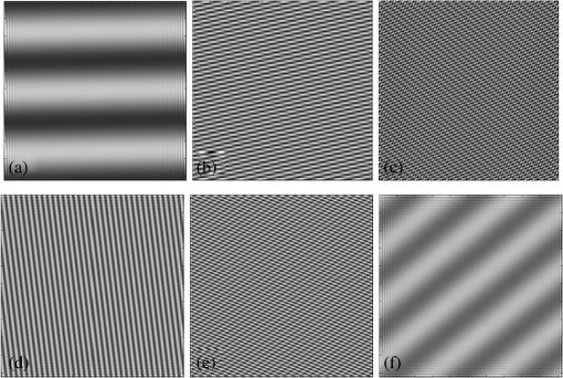
Examples of the moiré patterns are shown in Fig. 8; the corresponding gratings are shown in Fig. 7. Figure 8 shows the moiré patterns at the angles near the edges of the domain and near its middle for the size ratios of 1 and 0.707 (namely, the angles slightly deviated from 0 deg, 45 deg, and 27 deg). Note that the period of the patterns in Figs. 8(b)–8(e) is not much longer than the period of the gratings.

Let us find the intersection of the functions defined by Eqs. (19) and (20). Substitute ρ1ρ1 mentioned above into the first function, and ρ2ρ2 into the second one. At the intersection, the two functions are equal, i.e.,

Eq. (21)

√1−2cosα+1=√1−2√2cosα−2√2sinα+1,1−2cosα+1=1−22cosα−22sinα+1,

which is equivalent to the following equation:

Eq. (22)

cosα(1−sinα)=12.cosα(1−sinα)=12.

Fig. 8Download

Moiré patterns: size ratio 1, angles 2 deg, 27 deg, and 43 deg in (a), (b), and (c), respectively; size ratio 0.707 and the same angles in (d), (e), and (f), respectively.

For the new variable S=sinαS=sinα, Eq. (22) can be rewritten as a quartic equation

Eq. (23)

S4−2S3+2S−34=0.S4−2S3+2S−34=0.

This equation has the only real root S=0.442S=0.442 within the domain; the corresponding angle is

Eq. (24)

α0=26.261deg.α0=26.261deg.

Note that this angle is very close to

Eq. (25)

α1/2=arctan12=26.565deg.α1/2=arctan12=26.565deg.

(The difference between two above angles is about 1%). It means that either of two angles Eqs. (24) or (25) can be practically used in the sinusoidal approximation with the accuracy about 99%.

From a proper (long enough) distance, the short-period patterns at the angle α0α0 (or α1/2α1/2) are unrecognizable and thus are effectively eliminated, see Figs. 8(b) and 8(e). For the equations in the polar coordinates refer to Ref. 59.

3.2.1.

Exercises

• 1. Point out the terms of Eq. (15) responsible for the strongest functions given in Eqs. (19) and (20).

• 2. Write down the equation of strongest waves for the 60-deg rhomboidal grating combined with a line grating.

• 3. Find the period of residual moiré patterns at the optimal angle (you may use either of two branches).

• 4. Find the period of the moiré patterns in square grating 1 mm + line grating 1.1 mm at the angles of 0 deg, 5 deg, and 10 deg.

• 5. Determine the orientation of the moiré pattern in line gratings 1 mm + 1.2 mm installed at 10 deg.

Sinusoidal Noncoplanar Gratings

Practically, the layers may not lie in the same plane. For example, a typical structure of the autostereoscopic 3-D displays contains two parallel layers separated by an air gap. Such a nonplanar layout makes the moiré patterns alive and vivid. The visual picture may look dissimilar from different directions, and the movement of the patterns sometimes looks unexpected; moreover, their behavior may seem unpredictable. This section is based on Refs. 28 and 60. Consider two layers observed from a finite distance ll as shown in Fig. 9.

Fig. 9Download

Two noncoplanar layers and the observer.

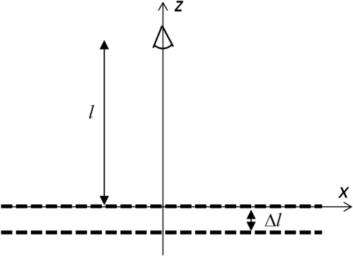
According to Ref. 60, the period of the moiré patterns in this case (two line gratings) is

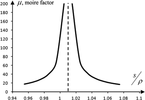
This expression for the period can be rewritten in terms of the moiré magnification factor; by its physical meaning, the moiré factor is an amplification coefficient (or a gain factor) for the period of the grating. The moiré factor corresponding to Eq. (26) is

Note that when ρ=sρ=s, the moiré factor Eq. (28) formally reaches infinity, which means the infinitely long period. However practically, we cannot measure an infinite period. The maximum value of the period is always limited by the size of a screen, where the patterns are observed; this is because the patterns with the period longer than that screen cannot be recognized as periodic waves at all. Equation (28) is graphically shown in Fig. 10.

Fig. 10Download

Moiré factor depending on ratio s/ρs/ρ.

The particular case of Eq. (28) for the identical gratings with ρ=1ρ=1 is as follows:

Examples of moiré patterns are shown in Fig. 11 for the same distance, but different gaps between gratings in Figs. 11(a) and 11(b), as well as for the same gap but different distances in Figs. 11(c) and 11(d).

Fig. 11Download

Moiré patterns in identical gratings. Computer simulation of gratings with period 0.11 cm at the same distance 100 cm, but different gaps: (a) 2 cm, (b) 5 cm; one unit = 1 cm. Experimental photographs of gratings with period 0.3 cm and the same gap 7 cm, but different distances: (c) 50 cm and (d) 100 cm.

A lateral displacement of the gratings (or the camera) does not affect the period; however in this case, the patterns are displaced laterally by the following value:

Note that our equations were obtained for the camera axis orthogonal to the plain gratings. The picture may look completely different in an nonorthogonal case. Compare two photographs of the same plane pavement in Fig. 12 taken by the same camera, but with the different angles between the camera axis and the surface.

Fig. 12Download

Two photographs of the same pavement taken by the same camera, but from different angles.

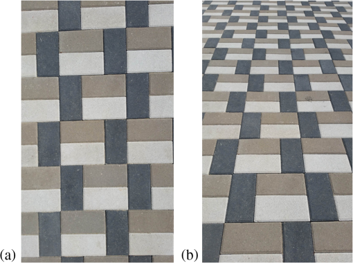
In the first case (the camera axis perpendicular to the surface), the shape and size of all bricks (rectangles) in the photograph are identical. In the second case (the camera with the axis deviated from the perpendicular), all quadrilaterals (projections of the rectangular bricks) are different; it means a strong dependence of their shape and size on coordinates.

Cylindrical Moiré (Orthogonal Projection)

Consider a regular 3-D object: a cylinder made of a wrapped periodic mesh, see Fig. 13. This section is based on Refs. 6162.–63.

Fig. 13Download

Cylinder observed through both halves.

The cylinder can be logically split into two halves, front and rear, which are made of the same mesh. When we look through meshes with a gap between them, the moiré patterns may appear, as described in Sec. 4.

To calculate the period of the moiré patterns, we use the orthogonal projection of the points lying on the surface of the cylinder onto a screen which is parallel to the xyxy-plane. Correspondingly, the projection lines are always parallel to the zz-axis; the coordinate xx can be treated as an impact parameter. Let RR be the radius of the cylinder, LL the distance from the screen SS to the center of the circle. An example projection line in Fig. 14 connects three circular dots, two on the circle, and one on the screen. The point, where this line crosses the xx-axis, is the orthogonal projection of two points from the cylindrical surface onto the screen SS.

Fig. 14Download

Horizontal cross section of cylinder.

In this section, all distances are measured along the lines parallel to the zz-axis. The distance ΔlΔl between the gratings along the zz-coordinate displaced by xx is equal to the chord of the circle. From the equation of the cylinder, the length of the chord is

Then, the distance ll from the observer to the first grating is LL minus one half of the chord

With using the polar angle φ=arcsin(x/R)φ=arcsin(x/R) of polar coordinates, Eqs. (31) and (32) can be re-expressed as follows:

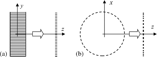
The variables ll and ΔlΔl for Eq. (29) describing the moiré effect in the parallel noncoplanar gratings are found. However in the case of a spatial object as a cylinder, the gratings are not parallel, and therefore the orientation of the wave vector in space has to be additionally taken into account. Correspondingly, two types of gratings on the surface of the cylinder should be analyzed: the grating with the vertical wave vector orthogonal to the base of the cylinder shown in Fig. 15(a) and the grating with the horizontal wave vector parallel to the base shown in Fig. 15(b).

Fig. 15Download

Wave vectors of two types of gratings on the cylinder (a) vertical wave vector and (b) horizontal wave vector.

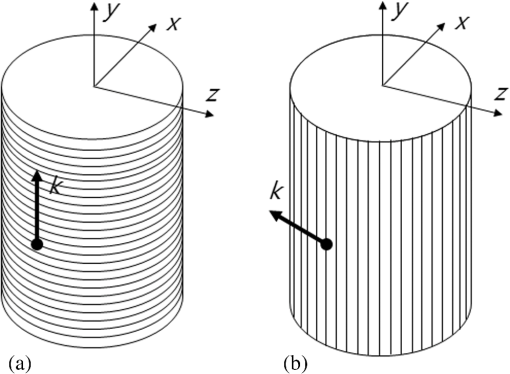
In the other words, the former grating consists of the identical circles uniformly displaced along the yy-axis; the latter consists of the vertical lines uniformly distributed along the circle, the base of the cylinder. These two cases are well separated (this fact is confirmed experimentally in Ref. 61) and therefore can be considered in isolation from one another.

In the orthogonal projection of the first grating onto the yzyz-plane, the projected period is equal to the period of the grating, see Fig. 16(a). However, the projected period of the second grating is not constant along the xx-axis, as shown in Fig. 16(b), and depends on the local inclination of the cylindrical surface, which is proportional to the cosine of the polar angle. Therefore in this case, the projected period should be multiplied by cosφcosφ.

Fig. 16Download

Orthogonal projections of two types of gratings onto the screen parallel to xyxy-plane: (a) vertical wave vector and (b) horizontal wave vector.

Based on Eqs. (33) and (34), the moiré periods of these cases are calculated as follows:

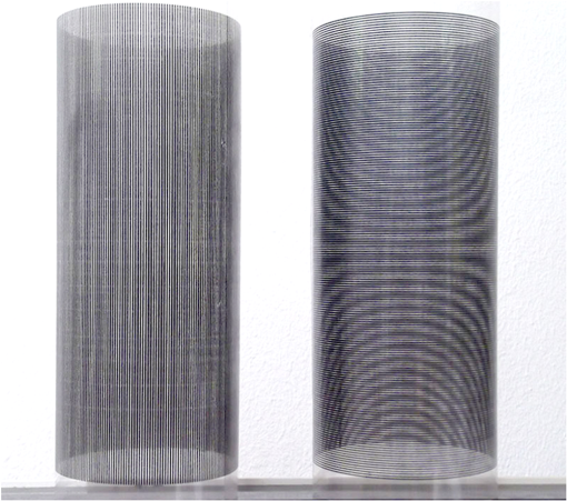
The photographs of the moiré patterns in cylinders with the horizontal and vertical wave vectors are shown in Fig. 17.

Fig. 17Download

Experimental photographs of the moiré patterns in two types of gratings.

The corresponding moiré magnification factors are given by the following equations:

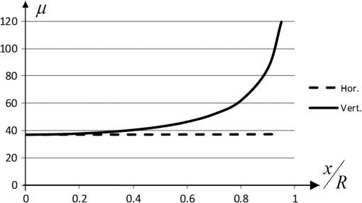
A graphical illustration of the theoretical dependences Eqs. (37) and (38) is shown in Fig. 18. Note that cosφ=x/Rcosφ=x/R. Across the radius, the horizontal moiré factor deviates <1%<1%, whereas the vertical one raises more than twice.

Fig. 18Download

Theoretical moiré factors in cylindrical objects for two orthogonal wave vectors (L/R=75L/R=75).

Moiré Wave Vector as a Vector Sum

Now, consider the moiré effect in the spectral domain, where we deal with the reciprocal distances or, equivalently, with the wave vectors.

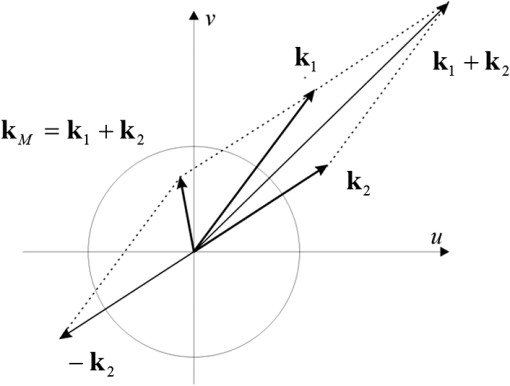
Generally speaking, the wave vector of the moiré patterns is that linear combination of the wave vectors of gratings (with coefficients +1+1 and −1−1), which is closest to the origin. It means either the sum or the difference; whichever is shorter, see Fig. 19. Typically (but not always), it is the difference between the wave vectors of two gratings.

Fig. 19Download

The moiré wave vector in two layouts of the wave vectors of gratings: (a) sum and (b) difference.

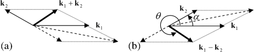
Let k1k1 and k2k2 be the wave vectors of the gratings and αα the angle between them. Based on these vectors, we will find the moiré wave vector kmkm and the moiré orientation angle θθ. Figure 19 is an illustration for the wave vectors with close wave numbers but different orientations.

It can be seen that for close wave numbers and α>90degα>90deg, it is the summation; otherwise (i.e., when α<90degα<90deg), it is the subtraction. Figure 19(b) actually shows the layout of the wave vectors for Eq. (10) in Sec. 3.

Figure 20 shows the map of the spectrum of two overlapped sinusoidal gratings [Fig. 19(b)]. Among all combinational components, the linear combination with the smallest wave number is the moiré wave vector.

Fig. 20Download

Map of spectrum (all linear combinations of wave vectors) of two overlapped sinusoidal gratings.

The extremely important concept of the visibility circle1 models the human visual system in the spectral domain. The visible vectors lie within the visibility circle, the vectors outside the visibility circle are invisible, see Fig. 21.

Fig. 21Download

Moiré wave vector and visibility circle.

Consider the triangle with the sides k1k1 and kmkm and the angle 2π−θ2π−θ between them in the case of the subtraction shown in Fig. 19(b). From the law of cosines for the side k2k2

From the law of cosines for the side kmkm, we have the modulus of the moiré wave vector

Therefore,

Recall that

Thus, the orientation of the wave vector of the moiré patterns is

The two Eqs. (41) and (46) comprise the full solution (the wave number and the orientation).

The relation for the periods is an inverse wave vector Eq. (41)

The orientation Eq. (46) can be also rewritten in terms of the periods

This is actually the same expression as Eq. (6) in Sec. 2. Moreover, Eqs. (47) and (48) can be re-expressed in terms of the ratio of periods ρ=T2/T1ρ=T2/T1 [compare with the definition Eq. (13) in Sec. 3.2] as follows:

Furthermore, Eq. (49) can be expressed in terms of the moiré factor

Basics of Two-Dimensional Fourier Transform

Spectra

A relation between variables can be described mathematically in two ways: either by the functional dependence or by the spectrum; corresponding examples are given in Fig. 22. Both ways characterize the same relation from different perspectives. For example, Figs. 22(a) and 22(b) describe the sinusoidal wave, whereas Figs. 22(c) and 22(d) the square wave.

Fig. 22Download

1-D functions (sinusoidal and square waves) and their power spectra: (a) sinusoidal function and (b) its spectrum of the right column, (c) square function, and (d) its spectrum of the right column.

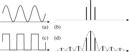
The Fourier spectra of real symmetric functions are real and symmetric, although in general, the spectra of arbitrary functions (including the real but nonsymmetric functions) are complex. In the tutorial we consider the power spectra, i.e., the modules of the Fourier coefficients, which are always real. For the periodic sinusoidal f1f1 and rectangular f2f2 functions shown in Fig. 22, we have

Eq. (52)

f1(x)=12+sinkx,f1(x)=12+sinkx,

Eq. (53)

⎧⎪⎨⎪⎩f2(x)={1,|x|<1/20,1/2<|x|<1f2(x+T)=f2(x),{f2(x)={1,|x|<1/20,1/2<|x|<1f2(x+T)=f2(x),

and the corresponding spectra are

Eq. (54)

F1(k)=12+δ(k)+δ(−k)4,F1(k)=12+δ(k)+δ(−k)4,

Eq. (55)

F2(k)=12+2π∞∑n=1,3,5,…1nsin(2πnk).F2(k)=12+2π∑n=1,3,5,…∞1nsin(2πnk).

The previous expression can be rewritten in terms of sinc function defined as follows:

Eq. (56)

sinc(x)=sin(x)x.sinc(x)=sin(x)x.

(Sometimes you can meet an alternative definition sinc(x)=sin(πx)/πxsinc(x)=sin(πx)/πx which differs in the normalization of the coordinate.) The rewritten Eq. (55) is as follows:

Eq. (57)

F2(k)=12+4k∞∑n=1,3,5,…sinc(2πnk).F2(k)=12+4k∑n=1,3,5,…∞sinc(2πnk).

The sinusoidal grating has three spectral components (one of them is a constant term, while two others represent a sinusoidal wave itself). The rectangular grating has many spectral components; theoretically, an infinite number of the decayed components. The decay rate of the Fourier coefficients depends on the smoothness of the function64 and particularly, for a piecewise continuous function is 1/n1/n. The spectrum of a symmetric square wave contains only odd harmonic frequencies, see Fig. 22(d), where all even harmonics are equal to zero. Figure 22(b) shows that the power spectrum of a sinusoidal grating can be thought as a limited (central) part of the spectrum of a rectangular grating.

Two-Dimensional Spectra

Figure 22 of the previous section shows the 1-D functions. A 1-D function of one variable (graphically, the “height” yy as a function of the abscissa xx) can be generalized to a 2-D function of two variables (the “height” zz as a function of two independent coordinates xx and yy).

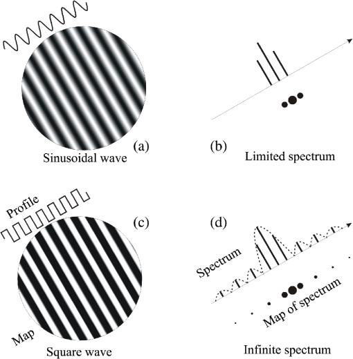
The 2-D case looks somewhat complicated, but not very sophisticated and still understandable. In two dimensions, the spectrum of a line grating is spread along a slant straight line (an abscissa of a 1-D spectrum) and repeated (copied) in the orthogonal direction. A 2-D function represents a surface and can be displayed, for instance, as a “map” with colors for the height; the white color may mean the lowest value (say, zero), while the black color means the highest value (say, one). Such maps of the plane waves (sinusoidal and square profile) are drawn in Figs. 23(a) and 23(c) together with their profiles; the spectra are shown in Figs. 23(b) and 23(d), respectively.

Fig. 23Download

2-D functions (sinusoidal and square waves) and their power spectra.

In many cases, a 2-D grid can be represented as a product of two 1-D gratings. For illustration, refer to Fig. 7 and to Eqs. (10) and (11). Many useful details about discrete transforms can be found in Ref. 56.

7.2.1.

Exercises

• 1. Describe the spectrum of the sinusoidal square grid (which is a superposition of two line gratings).

• 2. Describe the spectrum of the nonsinusoidal square grid.

• 3. Draw the map of peaks for three superposed sinusoidal gratings at the angle near 60 deg.

• 4. What is the 2-D Fourier transform of two orthogonal gratings with the periodic triangular transparency function?

• 5. How to find the phase of the wave from the Fourier coefficients?

• 6. Distance between the spectral peaks of the function sin(3x+4y)sin(3x+4y).

Spectral Trajectories

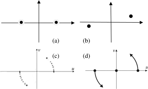
Generally speaking, parameters of the gratings do not always remain constant and may change. This change causes the change of the spectrum. In the case of an incremental change of a parameter, a set of several spectra represents a richer picture of the behavior of the patterns. For example, when a sinusoidal line grating whose initial spectrum is shown in Fig. 24(a) turned around, its spectrum is also rotated, see Fig. 24(b). Several overlapped spectra of an incrementally rotated grating are shown in Fig. 24(c) for the angles 0 deg to 40 deg with increment 5 deg; these look like a set of discrete points. Schematically, such sets of spectra can be drawn by continuous trajectories in the spectral domain, see Fig. 24(d).

Fig. 24Download

Spectra of one rotated grating (a) initial grating, (b) rotated grating, (c) overlapped spectra of grating rotated by several angles, and (d) scheme of spectra (spectral trajectory).

Furthermore, one may consider the spectral domain with the axes uu, vv as the complex plane with uu and vv as the real and the imaginary parts of a complex number zz. Then, all locations and shapes in the complex plane and spectral domain are identical, but the calculations become convenient and simple because the complex numbers allow applying many powerful mathematical theorems.

This section is based on Ref. 57. Consider a superposition of two rectangular grids, which can be often met in practice. The equation of the spectral peaks of four gratings arranged in two layers (each layer consists of two orthogonal gratings) is

A picture of trajectories Fig. 24(d) shows where the spectral peaks can be located when the angle varies. The spectral trajectories are known in many areas, refer, for instance, to Refs. 65 and 66. For the moiré effect, the spectral trajectories were first time proposed in Ref. 57.

In the case of two square gratings and the running angle, the trajectory derived from Eq. (58) is as follows:

It can be proven that the trajectories [Eq. (59)] are either circular arcs or segments of straight lines. Different dimensions of gratings (implying that a line grating is a 1-D structure, the square grid is a 2-D structure) yield two particular cases

The trajectories for two line gratings and two square grids [Eqs. (60) and (59)] are shown in Fig. 25. These trajectories were observed in experiments.57 Many examples of trajectories of the sinusoidal gratings for other running parameters can be found in Ref. 67.

Fig. 25Download

Trajectories [Eqs. (59) and (60)] for sinusoidal gratings (a) two line gratings and (b) two square grids. (Running angle αα between 5 deg and 40 deg, ρ=σ1=σ2=1ρ=σ1=σ2=1).

For the moiré effect, it is important that there can be trajectories leaving the visibility circle, approaching, entering, or crossing it, as well as the trajectories always outside or always inside the visibility circle. The visibility circle is shown in Fig. 25 by thin dashed line.

Visual Effects on the Move and on the Rotation

In the case of a laterally moved 1-D grating, the corresponding displacement of the visible moiré patterns is also lateral and given by Eq. (30) in Sec. 4. Similarly, the equation for displacement of the visible moiré patterns in the case of the moved observer can be derived from Ref. 60 as follows:

In both cases (the moved grating or the moved observer), the displacement of the moved object by one of its periods causes the displacement of the visual picture by one period of the moiré patterns. This visual picture repeats periodically. Correspondingly, the laterally moved observer will repeatedly see the same visual picture at each period of the patterns.

In the case of identical gratings (ρ=1ρ=1), we have from Eq. (62)

Equation (63) represents so-called moiré mirror effect in the identical gratings, which results in the displacement of the moiré patterns equal to the displacement of an observer; i.e., the patterns literally follow the observer’s movement, as his/her reflection in a plain mirror, see Fig. 26.

Fig. 26Download

Lateral displacement of the moiré patterns due to displacement of camera (a) on-axis camera, (b) off-axis (displaced) camera at the same distance. The patterns are shifted according to Eq. (63); the shift = lateral displacement of the observer.

When the gratings are turned around, i.e., the angle between the gratings changes, the period of the moiré patterns also changes. In the case of the sinusoidal square gratings, almost certainly there could be two maxima at 0 and at 45 deg. For nonsinusoidal gratings, there could be several maxima at the intermediate rational angles (whose tangents are rational numbers).

At the maxima, the axis of the moiré patterns is parallel to the axis of the rotated grating and their period is maximal.68 This can be explained in the following way. Although the spectral trajectory passes the neighborhood of the origin, the wave number reaches a minimum at that point, where the trajectory crosses the line connecting the origin and the center of the trajectory.

According to Eq. (26), the period remains finite for any relation between the parameters ρρ and ss, except for the case of ρ=sρ=s. In other words, the maximum period characterizes the relation between ρρ and ss. From this perspective, the value of the maximum magnification factor gives an estimate of this relation. Theoretically, the maximum period depends on the particular ratio of periods of the gratings, and for the coplanar gratings with the integer ratios, the period of the moiré patterns is infinite. There can exist several local maxima. For illustration, refer to the computer simulation.69

The moiré factor can only be infinite in the gratings with parallel wave vectors, when ρ=sρ=s, i.e.,

This means that to obtain the infinite moiré factor, the size should correspond to the distance and gap. Before and after the “critical” distance, the moiré factor is finite. When a long-distance observer approaches to the gratings, the moiré factor increases, then reaches infinity at the critical distance, and finally decreases.

In the identical gratings at zero angle (α=0α=0), the patterns are parallel to the gratings and the moiré factor is equal to z/dz/d.

In identical gratings (ρ=1ρ=1) with an arbitrary angle, both moiré factor and orientation vary as follows:

These equations mean that at a long distance, the moiré factor can be large, depending on the angle. When the observer approaches, the moiré factor drops down practically to zero, always remaining finite. On that move (approach), the moiré patterns rotate by ∼90deg∼90deg from almost orthogonal orientation to the parallel one.

These situations can be graphically illustrated as follows. The moiré factor in the identical gratings as a function of the distance under two conditions: d=constd=const with αα parameter is shown in Fig. 27; the graphs for α=constα=const with dd parameter look similar.

Fig. 27Download

(a) Moiré factor and (b) orientation in identical gratings. (The angle φφ in degrees.)

In nonidentical gratings, the moiré factor theoretically can reach the infinity. The cases of nonidentical gratings (with αα as parameter) and the parallel gratings (with ρρ as parameter) installed at the gap d=1d=1 are shown in Fig. 28. In the latter case, the moiré orientation is unchanged because practically we cannot distinguish between the directions 0 deg and 180 deg.

Fig. 28Download

(a) Moiré factor and (b) orientation in nonidentical gratings. Moiré factor (c) and orientation (d) in parallel gratings. (The angle φφ in degrees.)

The moiré factor and the orientation of the moiré patterns in the nonidentical gratings installed at a small angle are shown in Fig. 29.

Fig. 29Download

Moiré factor and orientation in nonidentical skew gratings in (a) and (b), respectively. (The angle φφ in degrees.)

Discussion and Conclusion

The tutorial covers several approaches to understand the moiré effect, to study it, and, particularly, to obtain the characteristics of the visible moiré patterns in the spatial and spectral domains. The physical meaning of equations is explained. The cross references between sections are made. The experimental evidences are provided in figures.

The following topics are covered: the indicial equation, the moiré wave vector, the sinusoidal coplanar and noncoplanar gratings, the moiré effect in the cylinder, as well as the 2-D Fourier transform, the moiré spectra, and the spectral trajectories. The visual effects in the displaced or rotated gratings are discussed. These topics collected in one article describe the moiré effect from various perspectives in a variety of scenarios. This gives readers a flexible opportunity to find solutions of practical problems using this or that approach.

For further reading, we would like to provide some additional references to the moiré effect in displays.70–72 Amazing, but the moiré effect, traditionally considered as a negative visual effect in displays, can be used to generate images including 3-D, refer to Refs. 38, 39, and 73. The color moiré effect is not considered in the tutorial. However, somebody interested can continue reading (Refs. 7475.76.77.–78).

As far as the gap effect is concerned, the paper28 is already mentioned. Some more papers on the gap effect must be mentioned, too, Refs. 7980.–81. The related moiré rotation effect is considered in Ref. 82.

Many sources on the moiré art are available.83–85 Among the books related to the moiré art, we would highly recommend the book,4 as well as a good interactive illustration.86 There are several modern painters and artists such as A. Minini, P. Dickens, P. Decrauzat, and C. Cruz-Diez, who use the moiré effect in their works; many of them are presented on the websites.87–90

The tutorial is intended for a wide audience, from beginners to specialists. Someone discovers the beauty of the moiré effect; someone finds details of the patterns, somebody else reveals a new approach. The authors believe that the tutorial can be useful for everybody who would read it.