thank for great post, anyone can help me, i done with entire code but just display only log result without gameplay of pong when running,
i run code with IDLE shell python 2.7.14 with my OS window 10 32 bit, what problem with me? i mean just only shell running and no gameplay of pong appeare ??

HI! @lucdaoinhan, add this command after gym.make("Pong-v0")

env = gym.wrappers.Monitor(env, '.', force=True)

Thanks for sharing great work :)
You really should have added your blog post url somewhere, which illustrates this code in really comprehensive way.

For anyone who may benefit, here is the link: http://karpathy.github.io/2016/05/31/rl/

I added a revision for Python 3.6.6 that works and it required more Mac setup that was in the original post:

git clone https://github.com/openai/gym.git; cd gym; brew install cmake boost boost-python sdl2 swig wget; pip install -e '.[atari]'

hey, I need some clear idea at line number 61. why we use 'epx'. can you write down backpropagation formula for w1 and w2.

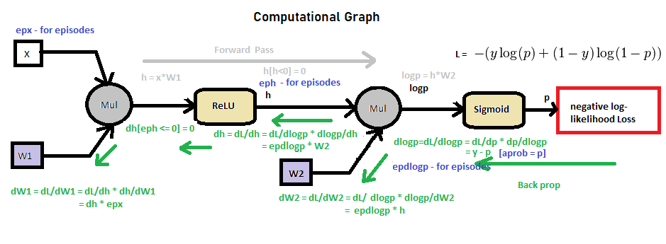
Here is the formula involved in the forward and backward functions, it appears clearly why the use of epx.

First, let's draw a picture of our neural network :

I used the general notation, but showed the corresponding values from the code (h and p).

What the forward function does is computing the following:

For the backward pass, we use the standard back propagation formula1, which are:

So we can use those to compute the gradients for W_1 and W_2.

For W_2:

Note we use the transpose of h to match the dimensions.

For W_1:

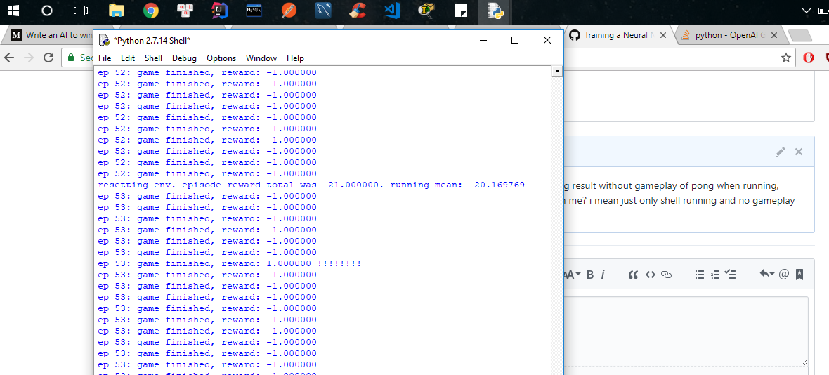
Last line... the position of the close bracket (parenthesis):
print ('ep %d: game finished, reward: %f' % (episode_number, reward) + ('' if reward == -1 else ' !!!!!!!!'))

HI, I have problem with the code can you help me
I am using python3.6 and it seem the code is wrong at this line
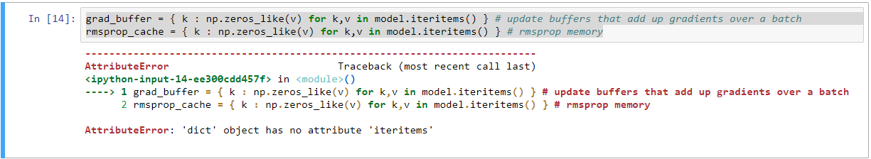
grad_buffer = { k : np.zeros_like(v) for k,v in model.iteritems() } # update buffers that add up gradients over a batch
rmsprop_cache = { k : np.zeros_like(v) for k,v in model.iteritems() } # rmsprop memory

the line
env=pygame.make(pong-n0).is wrong
it said the make attribute is not attribute of pygame

For anyone trying to understand the code in this gist, I found the following video from Deep RL Bootcamp really helpful, probably more helpful than Andrej's blog:

https://www.youtube.com/watch?v=tqrcjHuNdmQ

I made this code into a Colab Notebook running Python 3 that allows you to run this without local installation and keep training it. It also allows to display episodes played. I added some fixes/adjustments mentioned by several people in the comments here.

https://colab.research.google.com/github/DJCordhose/ai/blob/master/notebooks/rl/pg-from-scratch.ipynb

It performs ok after a few hours of training, but might take 1-2 days before it actually outperforms the computer player

I've forked the repo added some explanatory comments to the code, and fixed a minor bug which helps me to get a bit better performance (although this could be explained by randomness stumbling on a better reward return...

Basically the base repo trims off 35px from the start of the width of the input image, but only 15px off the end - which would mean the network is still training off when the ball passes the paddle, which isn't useful. Trimming more off the end of the image seemed to boost performance:

Using a learning rate of 1e-3 it took 12000 episodes to reach a trailing reward score of -5.
With the bugfix in place and a learning rate of 1e-3, the trailing average reward at 10000 episodes was 3ish

I had platform Win 64 bit , can this program work on it

@lucdaodainhan or just simply put render = True :)

HI, I have problem with the code can you help me
I am using python3.6 and it seem the code is wrong at this line
grad_buffer = { k : np.zeros_like(v) for k,v in model.iteritems() } # update buffers that add up gradients over a batch
rmsprop_cache = { k : np.zeros_like(v) for k,v in model.iteritems() } # rmsprop memory

Replace iteritems -->items.

grad_buffer = { k : np.zeros_like(v) for k,v in model.items() } # update buffers that add up gradients over a batch
rmsprop_cache = { k : np.zeros_like(v) for k,v in model.items() } # rmsprop memory

Hey guys,

I want to know how can I implement the policy gradient with baseline? Baseline seems to have its own calculation so I am getting confused how to put that in policy gradient.

Did anyone successfully implement the same thing in gym.retro Pong-Atari2600?

Hi, guys

Are all weights of the neural network increased by the same gradient. The gradient is a vector of the epoch, I think. We can add them to make them scalar. My question is are all parameters of the neural network being increased by the same scalar value. When we say theta=learning rate*gradient?

Or is the gradient partially derivated for every weight of the network.

Thanks for the code!

Thanks for the code.
Thank You guys for explaining many items related to back propagation.
Since no one has added a circuit diagram to visualize backprop, adding it here .It helped me to understand backprop in this code.

I want the paython code of neurel network where: input layer part is composed of two neurons, . The hidden layer is constituted of two under-layers of 20 and 10 neurons for the first under-layer and the second under-layer respectively. The output layer is composed of 5 neurons.

I want the python code of neural network where: input layer part is composed of two neurons, . The hidden layer is constituted of two under-layers of 20 and 10 neurons for the first under-layer and the second under-layer respectively. The output layer is composed of 5 neurons.

First, change the first hidden neuron size to 20 then the second hidden layers to 10. Using this u need to add new weights in the model dict object. Then use 'Xavier' initialization to initialize the weights. Then the last weight size u need to change it to 10x5. and everything else remains the same. First, u try implementing on your own and then everyone is here to help u with any errors and stuff
thank you

I have problem in updating weights
`import numpy as np

class Neural_Network(object):
def init(self):
#parameters
self.inputSize = 2
self.outputSize = 5
self.hiddenSize = 20
self.hiddenSize2 = 10

#weights
self.W1 = np.random.randn(self.inputSize, self.hiddenSize) # (2x20) weight matrix from input to hidden layer

print(self.W1)

self.W2 = np.random.randn(self.hiddenSize, self.hiddenSize2) # (20x10) weight matrix from hidden to output layer

print(self.W2)

self.W3 = np.random.randn(self.hiddenSize2, self.outputSize) # (10x5) weight matrix from hidden to output layer

print(self.W2)

def forward(self, X):
#forward propagation through our network
self.z = np.dot(X, self.W1) # dot product of X (input) and first set of 2x20 weights
self.z2 = self.sigmoid(self.z) # activation function
self.z3 = np.dot(self.z2, self.W2) # dot product of hidden layer (z2) and second set of 20x10 weights
self.z4 = self.sigmoid(self.z3) # final activation function
self.z5 = np.dot(self.z4, self.W3) # dot product of hidden layer (z2) and second set of 10x5 weights
o = self.sigmoid(self.z5) # final activation function
return o

def sigmoid(self, s):
# activation function
return 1/(1+np.exp(-s))

def sigmoidPrime(self, s):
#derivative of sigmoid
return s * (1 - s)

def backward(self, X, y, o):
self.o_error = y - o # error in output

self.o_delta = self.o_error*self.sigmoidPrime(o) # applying derivative of sigmoid to error

self.z3_error = self.o_delta.dot(self.W3.T) # z2 error: how much our hidden layer weights contributed to output error

self.W3 += self.z4.T.dot(self.o_delta) # adjusting second set (hidden --> output) weights


self.z3_delta = self.z3_error*self.sigmoidPrime(self.z3)


self.W2 +=0.001

self.W3 +=0.001

self.W1 +=0.001

def backprop(self):
# application of the chain rule to find derivative of the loss function with respect to weights2 and weights1
d_weights2 = np.dot(self.layer1.T, (2*(self.y - self.output) * sigmoid_derivative(self.output)))
d_weights1 = np.dot(self.input.T, (np.dot(2*(self.y - self.output) * sigmoid_derivative(self.output), self.weights2.T) * sigmoid_derivative(self.layer1)))

    # update the weights with the derivative (slope) of the loss function
    self.weights1 += d_weights1
    self.weights2 += d_weights2

def train(self, X, y):
o = self.forward(X)
self.backward(X, y, o)

def saveWeights(self):
np.savetxt("w1.txt", self.W1, fmt="%s")
np.savetxt("w2.txt", self.W2, fmt="%s")

def predict(self):

print ("Predicted data based on trained weights: ")

print ("Input (scaled): \n" + str(xPredicted))

print ("Output: \n" + str(self.forward(xPredicted)))

X = (hours studying, hours sleeping), y = score on test, xPredicted = 4 hours studying & 8 hours sleeping (input data for prediction)

X = np.array(([500, 10], [3700, 10], [500, 100], [3700, 100]), dtype=float)
y = np.array(([0.00512,0.0099,0.0051,0.952,0.1155], [0.0088,0.013,0.0101,0.62,0.1835], [890.00398,0.008,0.0034,1.109,0.0872],[0.00416,0.0163,0.0312,0.936,0.0947]), dtype=float)

#xPredicted = np.array(([4,8]), dtype=float)

scale units

#print(X)
X = X/np.amax(X, axis=0) # maximum of X array
y = y/np.amax(y, axis=0) # maximum of X array
#print(X)

#print(xPredicted)
#xPredicted = xPredicted/np.amax(xPredicted, axis=0) # maximum of xPredicted (our input data for the prediction)
#print(xPredicted)
#y = y/100 # max test score is 100
NN = Neural_Network()
for i in range(1000): # trains the NN 1,000 times
print ("# " + str(i) + "\n")
print ("Input (scaled): \n" + str(X))
print ("Actual Output: \n" + str(y))
print ("Predicted Output: \n" + str(NN.forward(X)))
print ("Loss: \n" + str(np.mean(np.square(y - NN.forward(X)))) )# mean sum squared loss
print ("\n")
NN.train(X, y)

NN.saveWeights()
#NN.predict()`

I'm trying to implement a model with Tensorflow following this gist. I'm trying to do it in a more general way to support cases where there can be more than 2 actions, so using sparse categorical cross entropy. I've been spending weeks on this, but can't make it work. Done all sorts of research, tried a lot of approaches (made 12 versions of it - surprisingly found a version which outperforms the original - using MSE for loss, and instead of subtracting the previous state from the current state, to get the state, it just uses the current state, but it should be just accidental luck), did lot of testing, but it performs terrible, actually, it doesn't learn at all.

Here's the code:

import tensorflow as tf
import numpy as np
import gym

class Model(tf.keras.Model):
  def __init__(self, h_units, y_size):
    super().__init__()

    self.whs = [tf.keras.layers.Dense(h_size, 'relu') for h_size in h_units]
    self.wy = tf.keras.layers.Dense(y_size, 'sigmoid')

  def call(self, x):
    for wh in self.whs:
      x = wh(x)
    y = self.wy(x)

    return y

def prepro(state):
  """ prepro 210x160x3 uint8 frame into 6400 (80x80) 1D float vector """
  state = state[35:195] # crop
  state = state[::2,::2,0] # downsample by factor of 2
  state[state == 144] = 0 # erase background (background type 1)
  state[state == 109] = 0 # erase background (background type 2)
  state[state != 0] = 1 # everything else (paddles, ball) just set to 1
  return state.ravel().reshape([1, -1])

class Environment:
  def __init__(self, state_preprocessor):
    self.env = gym.make('Pong-v0')
    self.state_preprocessor = state_preprocessor

    self.prev_s = None

  def init(self):
    cur_s = self.env.reset()
    cur_s = self.state_preprocessor(cur_s)

    s = cur_s - tf.zeros_like(cur_s)

    self.prev_s = cur_s

    return s

  def step(self, action):
    cur_s, r, done, info = self.env.step(action + 2)
    cur_s = self.state_preprocessor(cur_s)
    
    s = cur_s - self.prev_s

    self.prev_s = cur_s

    return s, r, done

# Runs model (policy) with x (input),
# samples y (action) from y_pred (probability of actions).
# Takes:
#  - x - the input, 1D tensor of the current state
#  - model - policy, returns probability of actions from state
#  - loss function to calculate loss
# Returns:
#  - gradients of model's weights based on loss
#  - loss from y, and y_pred with loss_fn
#  - y - 1D tensor, the sampled value what the action should be
@tf.function
def sample_action(x, model):
  y_pred = model(x)
  samples = tf.random.uniform([1])

  y = y_pred - samples
  y = tf.reshape(tf.argmax(y, 1), [-1, 1])

  return y

def get_gradients(x, y, r, model, loss_fn):
  with tf.GradientTape() as tape:
    y_pred = model(x)
    loss = loss_fn(y, y_pred, r)

  gradients = tape.gradient(loss, model.trainable_variables)

  return gradients

# Discounting later rewards more than sooner.
# Because the final reward happened much more likely
# because of a recent action than one at the beginning.
# Takes:
#  - full value rewards of timesteps
#  - discount multiplier
# Returns:
#  - discounted sum of rewards of timesteps

def discount_rewards(d):
  def discount(rs):
    d_rs = np.zeros_like(rs)
    sum_rt = 0
    for t in reversed(range(rs.shape[0])):
      if rs[t] != 0: sum_rt = 0
      # add rt to the discounted sum of rewards at t
      sum_rt = sum_rt * d + rs[t]
      d_rs[t] = sum_rt
    d_rs -= np.mean(d_rs)
    d_rs /= np.std(d_rs)
    return d_rs
  return discount

model = Model([200], 2)
env = Environment(prepro)
loss_fn = tf.keras.losses.SparseCategoricalCrossentropy(reduction=tf.keras.losses.Reduction.NONE)
optimizer = tf.keras.optimizers.RMSprop(0.0001, 0.99)
discounter = discount_rewards(0.99)

epochs = 10000
batch_size = 10

# Train runs the model with the environment,
# collects gradients per execution, and optimizes
# the model's weights at each epoch.
# Takes:
#  - model (policy), which takes the input x (state), and returns y (action)
#  - environment, which performs the action, and returns the new state, and reward
#    must have methods:
#     - init() - initialize the state
#     - step(action) - perform the action, return new state, reward, and indicator if episode is over

def train(model, env, loss_fn, optimizer, discounter, epochs, batch_size):
  for i in range(epochs):
    xs = []
    ys = []
    rs = []
    ep_rs = []

    for e in range(batch_size):
      done = False
      x = env.init()
      ep_r = 0

      while not done:
        xs.append(x)
        y = sample_action(x, model)
        ys.append(y)

        x, r, done = env.step(y.numpy().astype('int'))
        rs.append(r)

        ep_r += r
      ep_rs.append(ep_r)
      print('Epoch:', i, 'Episode:', e, 'Reward:', ep_r)
    
    xs = tf.concat(xs, 0)
    ys = tf.concat(ys, 0)
    rs = np.vstack(rs)
    rs = discounter(rs)

    gradients = get_gradients(xs, ys, rs, model, loss_fn)
    optimizer.apply_gradients(zip(gradients, model.trainable_variables))

    print('Epoch:', i, 'Avg episode reward:', np.array(ep_rs).mean())

train(model, env, loss_fn, optimizer, discounter, epochs, batch_size)

So in summary, set up a model with 2 dense layers, output the number of possible actions, subtract the random number from the output, get the index of the highest one, use it as the action. Run the environment with it, get the next state, and reward. Store all selected actions, rewards, states. If the number of episodes reach the batch size, rerun the model with the collected states, get the predictions, run sparse categorical cross entropy with the selected actions, and predictions, use the discounted rewards as sample weights for the losses, get the gradients, optimize the weights. Repeat.

During making those versions, and testing them, I realized that somehow the initial version makes a lot better random guesses before any training (10 episodes) with a mean of 20, while the tensorflow version keeps guessing -21 for all 10 episodes in multiple independent tries.

All makes sense, but doesn't work. Why?

@Grsz That is a perfect question for StackOverflow...

Python3 version of pg-pong.py with the minimum changes to make it work:
https://gist.github.com/haluptzok/d2a3eba5d25d238d6c2cbe847bc58b6b
Still a great policy gradient blog post and python script - but Python2 is so 2016 : )
Most folks reading this now will fire it up in python3 and blow up and not get the fun experience

For those interested in seeing this implemented on top of TensorFlow 2 running entirely on graph mode here's the repo:

https://github.com/WillianFuks/Pong

The AI trained fairly quickly, in a day it already reached average return of ~14 points. But then it stops there and doesn't quite improve much after all. Not sure on how to further improve it then, other than keep tweaking the hyperparams.

May 19th 2022
I modify some lines of pg-pong.py because this is too old (but gold).
In my case rendering option did not work because of openai-gym issue.
pls check this code if you want to train agent playing pong in py38, gym>=0.21.0

In case someone wants to share a cool colab demo still - here is my notebook that ended up achieving level performance with the human opponent
https://colab.research.google.com/drive/1KZeGjxS7OUHKotsuyoT0DtxVzKaUIq4B?usp=sharing