Your Friends Have More Friends Than You

Vishesh Khemani, Ph.D. on 2021-03-04

Getting Started

A friendly introduction to the Friendship Paradox

An Unfriendly Truth

Your friends most likely have more friends than you do. You may find this humbling, hurtful, improbable, impossible, or simply quaint. But it’s the truth.

What exactly does it mean for your friends to have more friends than you? Suppose you have N friends. And your first friend has F₁ friends, your second friend has F₂ friends, and so on. Then, the average number of friends each of your friends has is <F> = (F₁ + F₂ + …) / N. For most of you, the average number of friends each of your friends has (i.e. <F>) is greater than the number of friends you have (i.e. N).

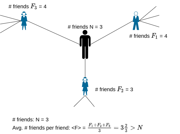
✍︎Image by author

The ego-bruising doesn’t stop there. Your lower connectivity relative to your connections is true for just about any network that you’re a part of. For example, on Twitter or Medium, your followers have more followers than you. Or, on LinkedIn, your connections have more connections than you. Or, if you’re a researcher, your collaborators on papers that you’ve published have more collaborators than you.

Even networks of non-sentient entities suffer this phenomenon. Most web pages are less prominent than the web pages they link to. Most research papers are cited fewer times than the papers they themselves cite.

How can this be? And is it just a theoretical curiosity, or does it have a more practical import?

Why Are You Less Popular Than Your Friends?

Model a network as a graph. For example, in a friendship network, each individual is a node (or vertex) in a graph. And if two individuals are friends then there’s an edge (or link) connecting the nodes of the two individuals.

Here’s an example graph denoting a network of 6 people (unimaginatively named A, B, C, D, E, F) in which each person is friends with exactly 2 other people:

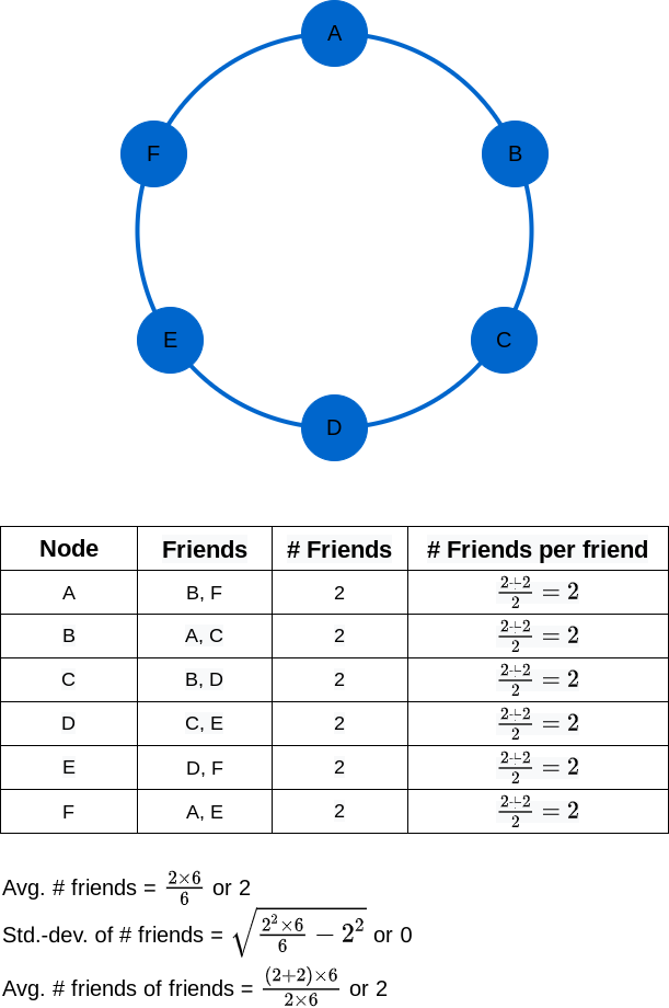
✍︎Image by author

In this example, each of the 6 people has 2 friends. And, each of the 2 friends of a person has 2 friends themselves. So, every person has the same number of friends as the number of friends each of their friends has. That’s quite a mouthful. And it doesn’t even manifest the property of most people having fewer friends than their friends. What gives? Well, unlike this example, real networks are not homogeneous. In other words, in real networks, the number of connections is not the same for every node. Furthermore, there are a small number of outliers nodes that are much more connected than the rest of the nodes. Let’s add one such outlier, Z, to the example graph:

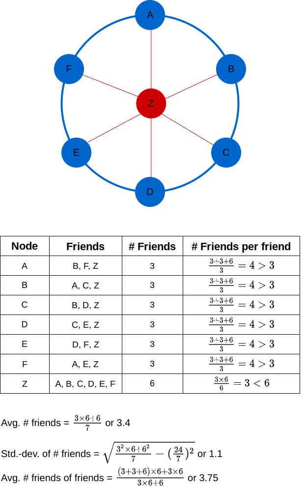
✍︎Image by author

Now, each of A to F has 3 friends. And Z has 6 friends. For each of A to F, 2 friends have 3 friends and 1 has 6 friends, making it an average of (3 + 3 + 6) / 3 or 4 friends per friend. So each of A to F is less popular than their friends. Only Z is more popular than their friends. Each of Z’s 6 friends has 3 friends. So Z’s friends have an average of 3 friends, whereas Z has 6 friends. The outlier Z skews the results for everyone else, and they become less popular than their friends.

In general, if a network has a fraction f of the nodes being much more highly connected than the rest of the nodes, then close to 1-f of the nodes in the network will be less connected than their connections. And most real-world networks, especially social ones, have a small fraction of nodes which are highly-connected outliers.

We can tighten the hand-waving with a precise mathematical result. If μ is the average number of connections per node in a network and σ is the standard deviation of the number of connections per node, then the average number of friends of friends is exactly μ + σ²/μ, which is greater than μ as long as there is some variation in the number of connections across the nodes. So, any heterogeneous network has a higher average number of friends of friends than of friends.

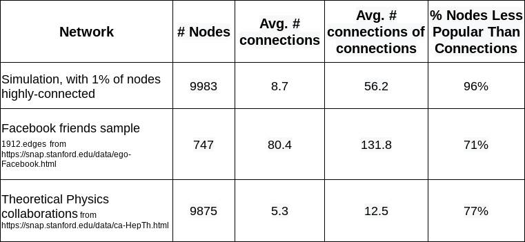
The following table shows three examples of this phenomenon. The first example is a randomly simulated network in which 99% of the nodes are typically connected and 1% of the nodes are highly connected. The second example uses data from a small subset of the Facebook friendship network. The third example uses the full data of all research collaborations in the Theoretical Physics preprint archives. In all three cases, the average number of connections of connections is greater than the average number of connections. And a large percentage of nodes are less connected than their connections.

✍︎Simulation and computation by author

Phone A Friend

Now that you’re resigned to the fact that your friends are more popular than you, you can shrug and move on. Or, you can read on to see how to harness this knowledge.

Suppose you want to influence the spread of something that is propagated locally between connected nodes in a network. For example, information spread in a community by face-to-face conversations, or an infectious disease spread in a population by physical contact. If you knew which nodes in the network are the most highly connected, you can surely use that to influence the spread. For example, to propagate information as fast as possible, seed the most highly connected nodes with the information. But, in reality, you don’t usually have visibility into such detailed knowledge of the network topology. In that case, a simple alternative is to seed a random sample of nodes and hope for the best. But, armed with the knowledge in this article, you can do a lot better with a “phone-a-friend” strategy: instead of seeding a randomly sampled node, seed a random connection of that node. Why does this make sense? Because we now know that a connection of a node is more likely to have more connections than the node itself. Does this really work? Absolutely. I’ll demonstrate with three examples.

Fast Gossip

Suppose you want to seed a piece of information among a small number of people in a community and rely on gossip among the community members for that information to spread. How do you pick the seed group of people so that the information spreads quickly? Use the phone-a-friend strategy. Choose a random set of people, but don’t seed them with the information. Instead, ask each person in the random set to nominate one of their friends. Then seed the nominated friends with the information.

✍︎Image by author

The graph above shows the result of a simulation. The lines show the cumulative percentage of people “infected” (i.e. received the information) as the gossip rounds progressed. The blue line is the base case of seeding a random 1% of the nodes. The red line shows the spread after seeding a random friend of each node from a random 1% of nodes. Clearly, the red line shows a faster spread of information after each round of gossip. After the first round, the information spreads to 12% (compared to the baseline of 3%). After the second round, it spreads to 43% (compared to the baseline of 20%). And so on.

If you’re interested, here are more details on the simulation (otherwise feel free to skip this). I constructed a random graph of 10,000 nodes in which 99% of the nodes had a smallish affinity to connect with other nodes (~2%) and 1% of the nodes had a high affinity to connect with other nodes (~71%). This produced a graph in which the average number of connections for a node was ~9, the average number of connections of connections was ~56, and 96% of the nodes had fewer connections than their connections. The spread of information was simulated in the following way: in one round of gossip, each person who has the information gossips it to a random quarter of their connections and then gets bored of it so that they don’t spread it in the next round of gossip.

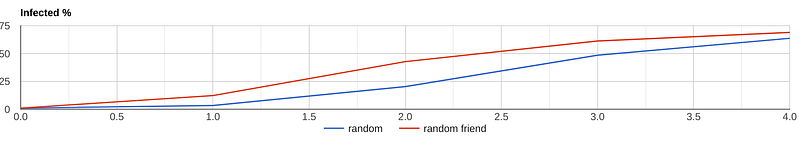
Early Detection

How can you quickly detect the spread of an infectious disease through a community by monitoring a small fraction of people in the community? Monitor a random friend of each person in a random sampling. Since a person’s friend typically has more friends than the person, the disease should show up faster among the people monitored under the phone-a-friend strategy.

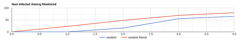✍︎Image by author

The graph above shows the result of a simulation. The lines show the number of monitored people who caught the infection as the disease spread through the community. The blue line is the base case of monitoring a random 1% of the people. The red line is the case of monitoring a random friend of each person from a random 1% selection of people. Clearly, the red line shows that by monitoring friends of a random sampling, the spread can be detected much earlier than by monitoring a random sampling. After the first round, 23 of the monitored friends were infected (compared to 0 in the baseline). After the second round, the disease could be detected in 48 of the random friends (compared to the baseline of 16). And so on.

Selective Immunization

Here’s a very relevant scenario for these times of a global pandemic with the need to prioritize whom to vaccinate. If there are only enough vaccines for a small fraction of the population, an effective strategy is to vaccinate a random friend of each randomly chosen person.

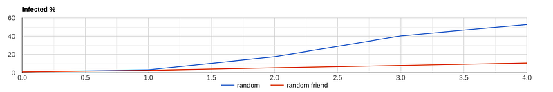✍︎Image by author

The graph above shows the result of a simulation. The lines show the cumulative percentage of people who caught the infection, starting with a random 1% of the people infected. The blue line is the base case of inoculating a random 10% of the people. The red line is the case of vaccinating a random friend of each person from a random 10% selection of people. The red line shows that the phone-a-friend strategy significantly reduces the spread. By the second round, the disease spread to only 5% of the people (compared to 17% in the baseline). By the third round, it spread to 8% (compared to the baseline’s 40%).

Summary

1. In a network which has some variance, σ², in the number of connections across nodes, the average number of connections per node, μ, is less than the average number of connections of connections by an amount σ² / μ.
2. If a network has a small number of highly-connected nodes, most of the other nodes have fewer connections than the average number of connections their connections have. So, for example, in a friendship network, a typical person will have fewer friends than the average number of friends their friends have.
3. The higher average connectivity of a connection of a node compared to the node itself can be used to influence the local propagation of information/infection in a network using a phone-a-friend strategy. Randomly sample a small set of nodes in the network (the baseline sample). Replace each node in the sampled set with a random connection of the node (the friends sample). The friends sample will be more highly connected than the baseline sample. If you seed the friends sample with some information ripe for gossip, it will spread much more rapidly than if you seed the baseline sample. If you monitor the friends sample for the spread of an infectious disease, you will detect it much earlier than if you monitor the baseline sample. If you immunize the friends sample against an infectious disease, you will significantly slow down the spread of the disease than if you immunize the baseline sample.

References