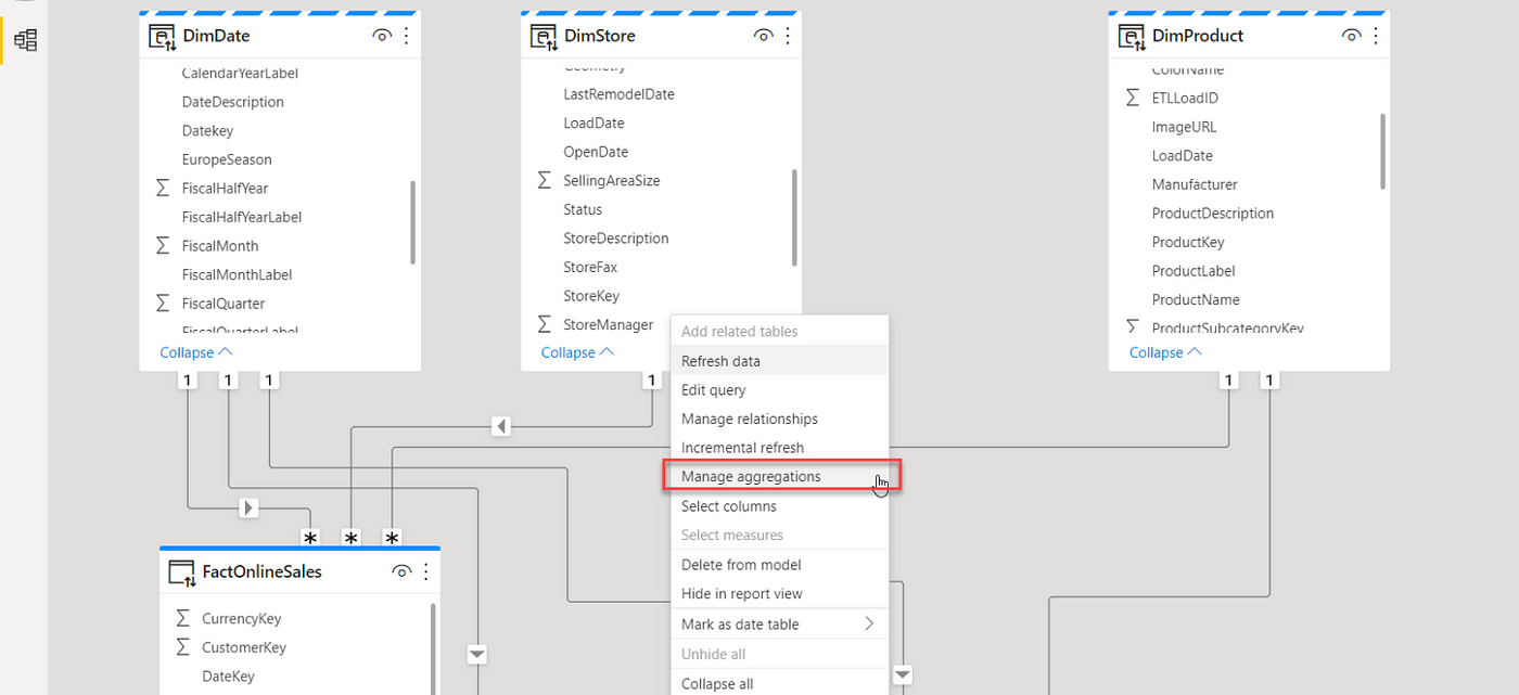
Image by author

In the previous article, while explaining the Composite models feature, we laid a solid ground for another extremely important and powerful concept — Aggregations! It’s because in many scenarios, especially with enterprise-scale models, aggregations are a natural “ingredient” of the composite model.

However, as composite models feature can be also leveraged without aggregations involved, I thought that it would make sense to separate these two concepts in separate articles.

Before we explain how aggregations work in Power BI and take a look at some specific use cases, let’s first answer the following questions:

Why do we need aggregations in the first place? What is the benefit of having two tables with identical data in the model?

Before we come to clarify these two points, it’s important to keep in mind that there are two different types of aggregations in Power BI.

• User-defined aggregations were up until a few months ago the only aggregation type in Power BI. Here, you are in charge of defining and managing aggregations, even though Power BI later automatically identifies aggregations when executing the query.
• Automatic aggregations are one of the newer features in Power BI and they have just recently been released as generally available feature. With the automatic aggregations feature enabled, you can grab a coffee, sit and relax, as machine learning algorithms will collect the data about the most frequently running queries in your reports and automatically build aggregations to support those queries.

The important distinction between these two types, of course besides the fact that with Automatic aggregations you don’t need to do anything except to turn this feature on in your tenant, is licensing limitations. While User-defined aggregations will work with both Premium and Pro, automatic aggregations at this moment require a Premium license.

From now on, we will talk about user-defined aggregations only, just keep that in mind.

Ok, here is a short explanation of aggregations and the way they work in Power BI. Here is the scenario: you have a large, very large fact table, which may contain hundreds of millions, or even billions of rows. So, how do you handle analytical requests over such a huge amount of data?

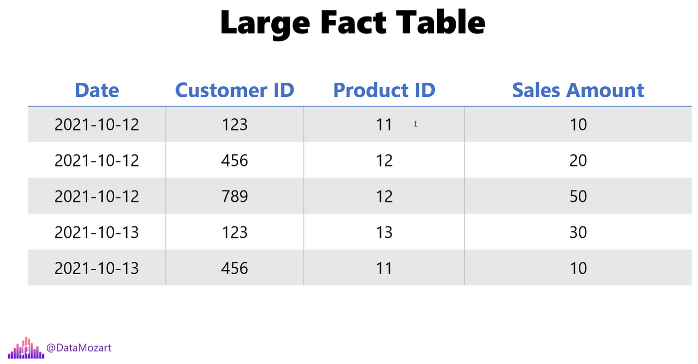
Image by author

You simply create aggregated tables! In reality, it is a very rare situation, or let’s say it’s more of an exception than a rule, that the analytic requirement is to see the individual transaction, or individual record as the lowest level of detail. In most scenarios, you want to perform analysis over summarized data: like, how much revenue we had on a specific day? Or, what was the total sales amount for product X? Further, how much did customer X spent in total?

Additionally, you can aggregate the data over multiple attributes, which is usually the case, and summarize the figures for a specific date, customer, and product.

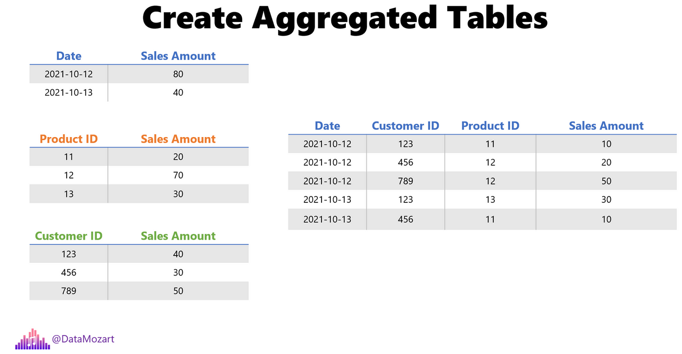
Image by author

If you’re wondering what’s the point in aggregating the data…Well, the final goal is to reduce the number of rows and consequentially, reduce the overall data model size, by preparing the data in advance.

So, if I need to see the total sales amount spent by customer X on product Y in the first quarter of the year, I can take advantage of having this data already summarized in advance.

Key “Ingredient” — Make Power BI “aware” of the aggregations!

Ok, that’s one side of the story. Now comes the more interesting part. Creating aggregations per-se is not enough to speed up your Power BI reports — you need to make Power BI aware of aggregations!

Just one remark before we proceed further: aggregation awareness is something that will work only, and only if the original fact table uses DirectQuery storage mode. We’ll come soon to explain how to design and manage aggregations and how to set the proper storage mode of your tables. At this moment, just keep in mind that the original fact table should be in DirectQuery mode.

Let’s start building our aggregations!

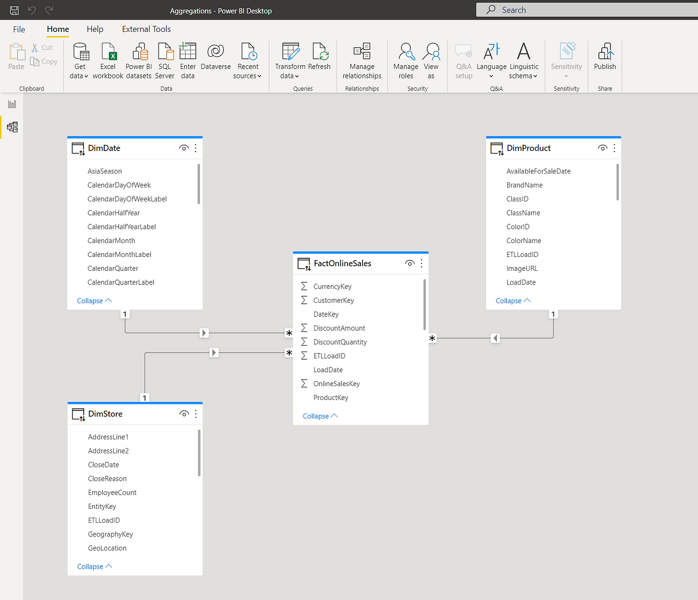
Image by author

As you may see in the illustration above, our model is fairly simple — consisting of one fact table (FactOnlineSales) and three dimensions (DimDate, DimStore, and DimProduct). All tables are currently using DirectQuery storage mode.

Let’s go and create two additional tables that we will use as aggregated tables: the first one will group the data on date and product, while the other will use date and store for grouping:

/*Table 1: Agg Data per Date & Product */
SELECT DateKey
       ,ProductKey
       ,SUM(SalesAmount) AS SalesAmount
       ,SUM(SalesQuantity) AS SalesQuantity 
FROM FactOnlineSales 
GROUP BY DateKey
        ,ProductKey/*Table 2: Agg Data per Date & Store */
SELECT DateKey
       ,StoreKey
       ,SUM(SalesAmount) AS SalesAmount
       ,SUM(SalesQuantity) AS SalesQuantity 
FROM FactOnlineSales 
GROUP BY DateKey
        ,StoreKey

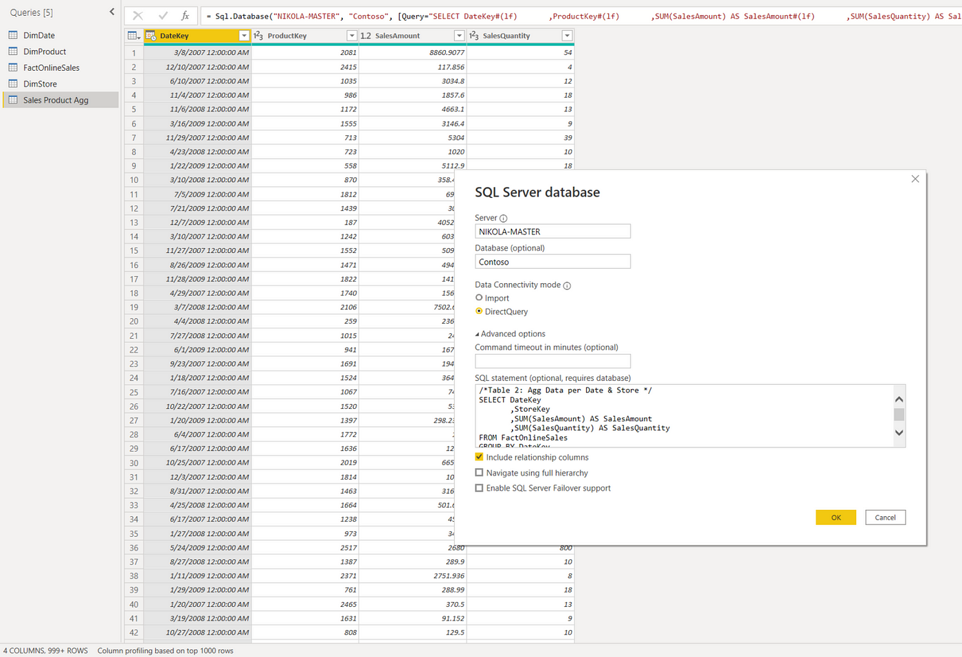
Image by author

I’ve renamed these queries to Sales Product Agg and Sales Store Agg respectively and closed the Power Query editor.

As we want to get the best possible performance for the majority of our queries (these queries that retrieve the data summarized by date and/or product/store), I’ll switch the storage mode of the newly created aggregated tables from DirectQuery to Import:

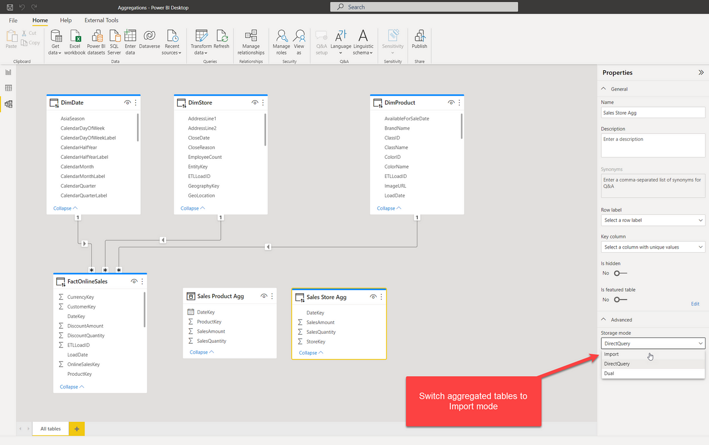
Image by author

Now, these tables are loaded into cache memory, but they are still not connected to our existing dimension tables. Let’s create relationships between dimensions and aggregated tables:

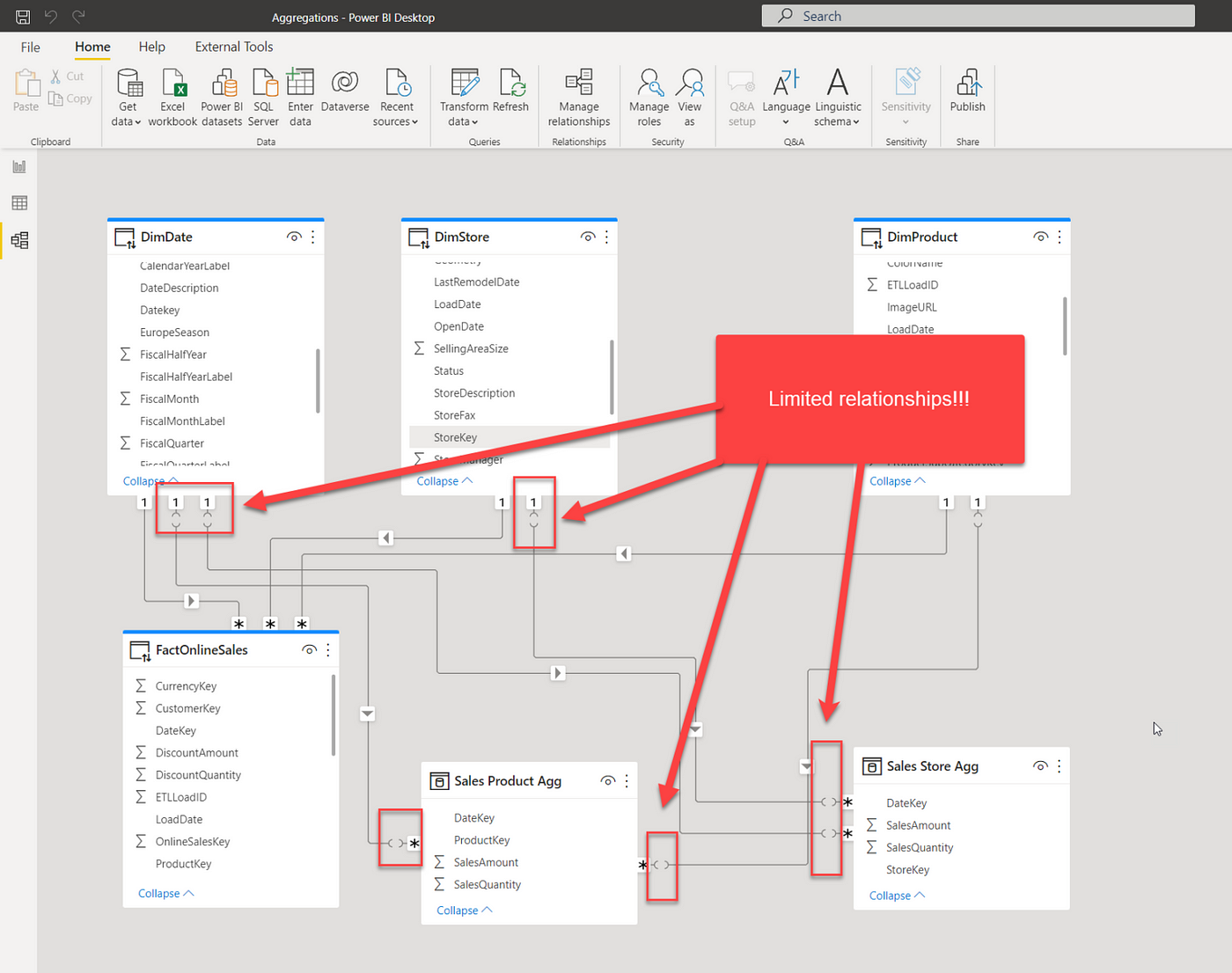
Image by author

Before we proceed, let me stop for a moment and explain what happened when we created relationships. If you recall our previous article, I’ve mentioned that there are two types of relationships in Power BI: regular and limited. This is important: whenever there is a relationship between the tables from different source groups (Import mode is one source group, DirectQuery is another), you will have a limited relationship! With all its limitations and constraints.

But, I have good news for you! If I switch the storage mode of my dimension tables to Dual, that means that they’ll be also loaded into cache memory, and depending on which fact table provides the data at the query time, dimension table will behave either as Import mode (if the query targets Import mode fact tables), or DirectQuery (if the query retrieves the data from the original fact table in DirectQuery):

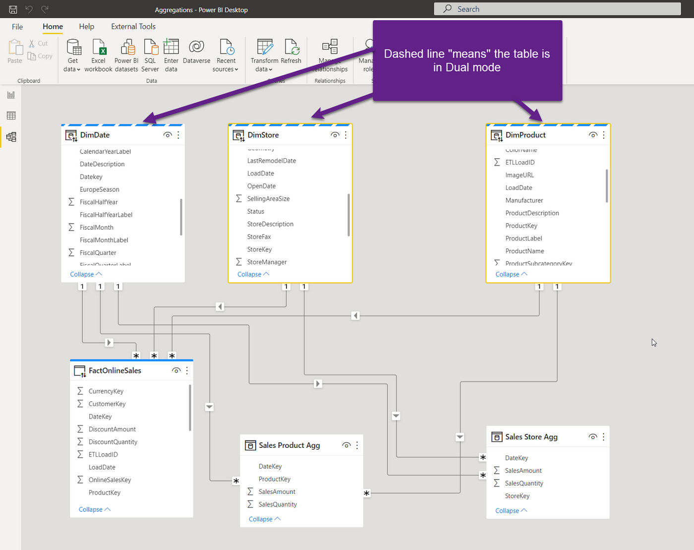
Image by author

As you may notice, there are no more limited relationships, which is fantastic!

So, to wrap up, our model is configured as follows:

• The original FactOnlineSales table (with all the detailed data) — DirectQuery
• Dimension tables (DimDate, DimProduct, DimStore) — Dual
• Aggregated tables (Sales Product Agg and Sales Store Agg) — Import

Awesome! Now we have our aggregated tables and queries should run faster, right? Beep! Wrong!

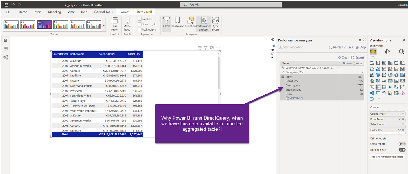
Image by author

Table visual contains exactly these columns that we pre-aggregated in our Sales Product Agg table — so, why on Earth does Power BI runs a DirectQuery instead of getting the data from the imported table? That’s a fair question!

Remember when I told you in the beginning that we need to make Power BI aware of the aggregated table, so it can be used in the queries?

Let’s go back to Power BI Desktop and do this:

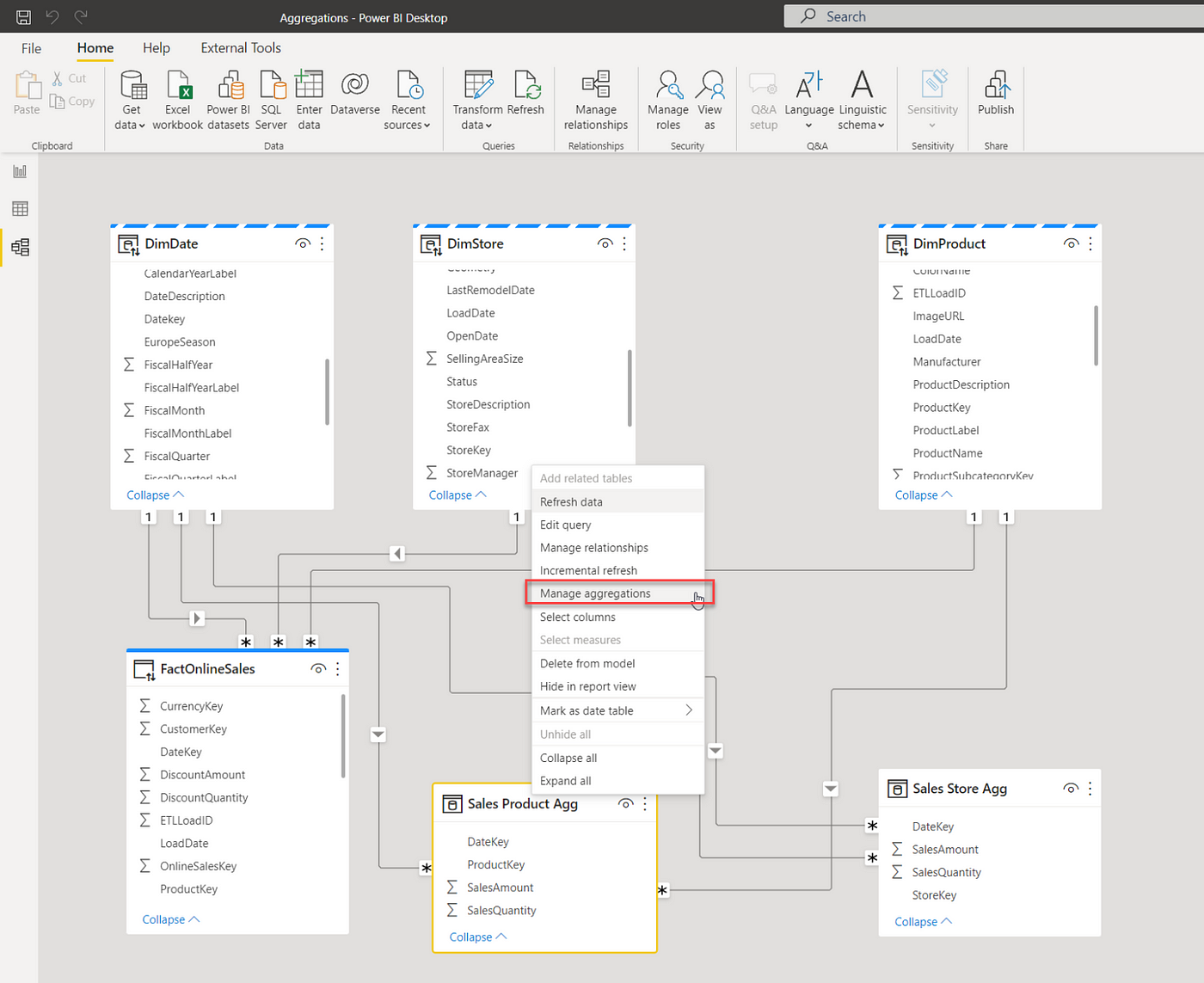
Image by author

Right-click on the Sales Product Agg table and choose the Manage aggregations option:

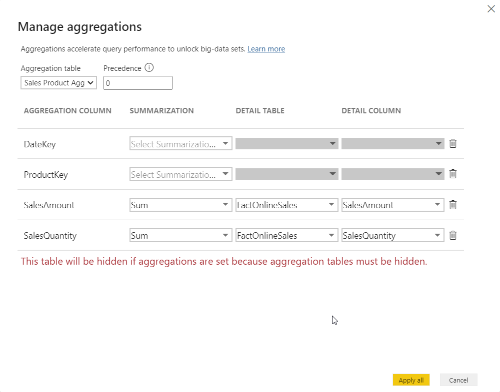
Image by author

A few important remarks here: in order for aggregations to work, data types between the columns from the original fact table and aggregated table must match! In my case, I had to change the data type of the SalesAmount column in my aggregated table from “Decimal number” to “Fixed decimal number”.

Additionally, you see the message written in red: that means, once you create an aggregated table, it will be hidden from the end-user! I’ve applied exactly the same steps for my second aggregated table (Store), and now these tables are hidden:

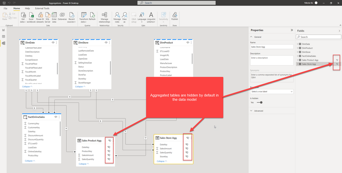
Image by author

Let’s go back now and refresh our report page to see if something changed:

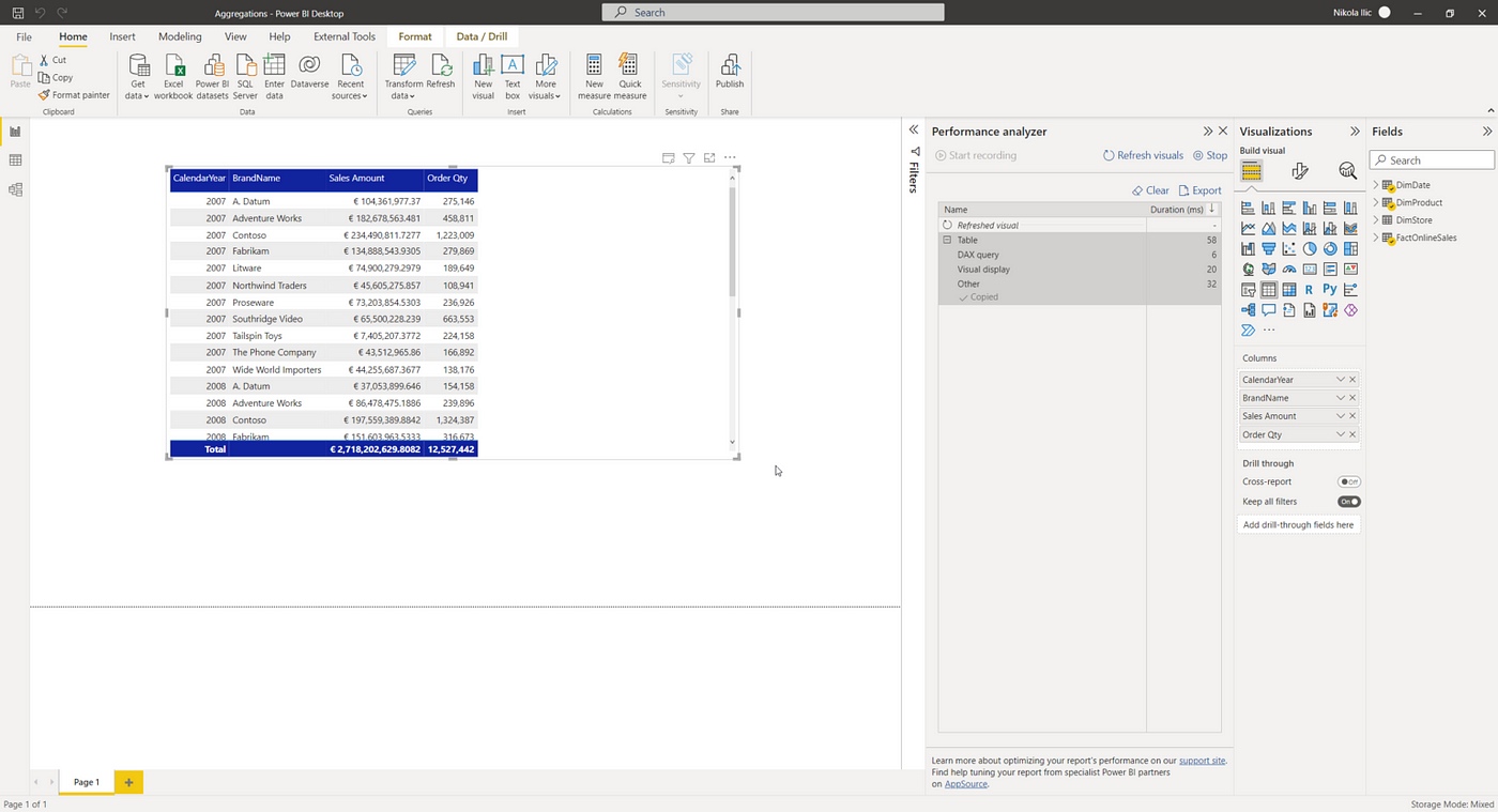
Image by author

Nice! No DirectQuery this time, and instead of almost 2 seconds needed to render this visual, this time it took only 58 milliseconds! Moreover, if I grab the query and go to DAX Studio to check what’s going on…

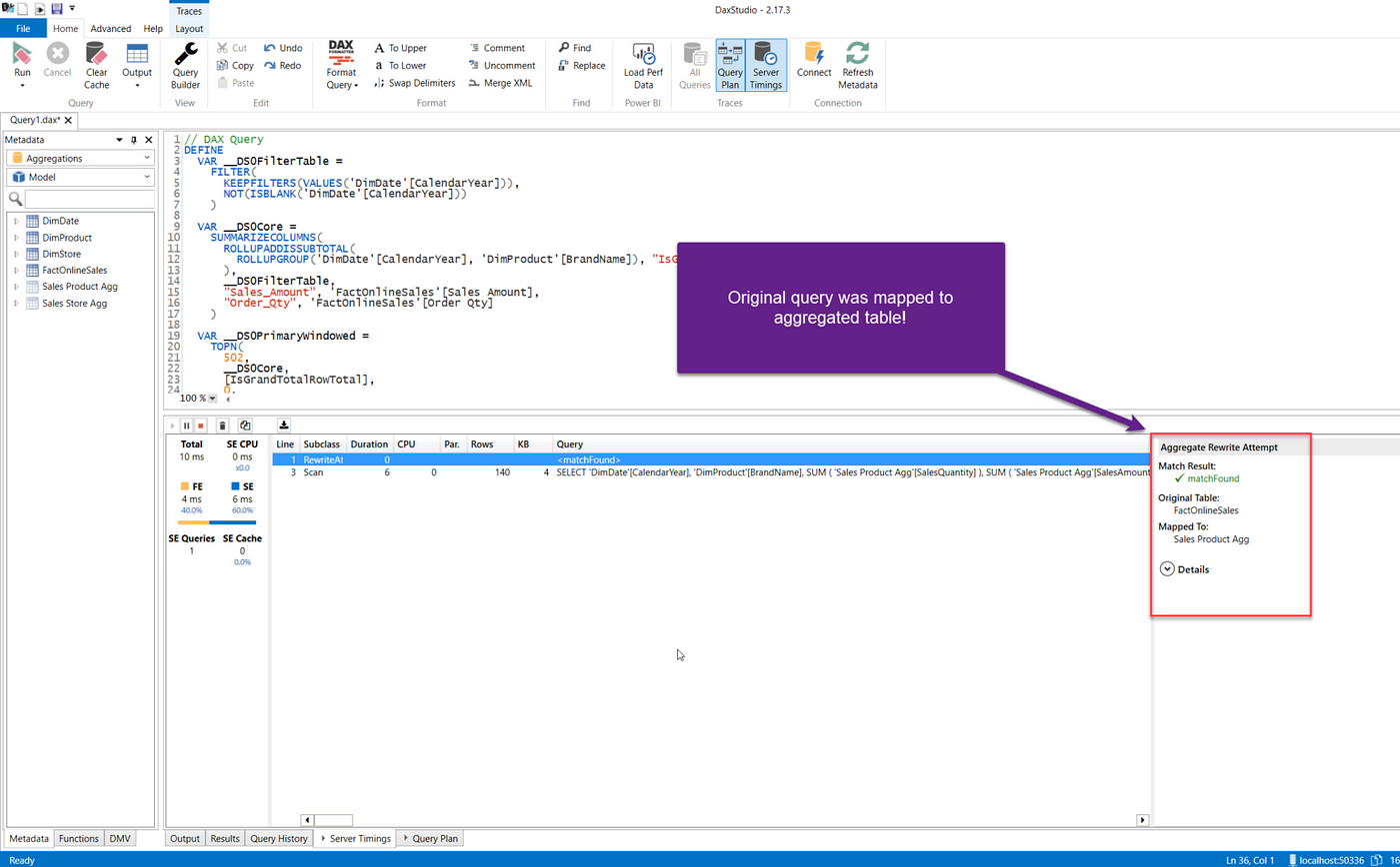
Image by author

As you see, the original query was mapped to target the aggregated table from import mode, and the message “Match found” clearly says that the data for the visual came from the Sales Product Agg table! Even though our user doesn’t have a clue that this table even exists in the model!

The difference in performance, even on this relatively small dataset, is huge!

Multiple aggregated tables

Now, you’re probably wondering why I’ve created two different aggregated tables. Well, let’s say that I have a query that displays the data for various stores, also grouped by date dimension. Instead of having to scan 12.6 million rows in DirectQuery mode, the engine can easily serve the numbers from the cache, from the table that has just a few thousand rows!

Essentially, you can create multiple aggregated tables in the data model — not just combining two grouping attributes (like we had here with Date+Product or Date+Store), but including additional attributes (for example, including Date and both Product and Store in the one aggregated table). This way, you’ll increase the granularity of the table, but in case your visual needs to display the numbers both for product and store, you’ll be able to retrieve results from the cache only!

In our example, as I don’t have pre-aggregated data on the level that includes both product and store, if I include a store in the table, I’m losing the benefit of having aggregated tables:

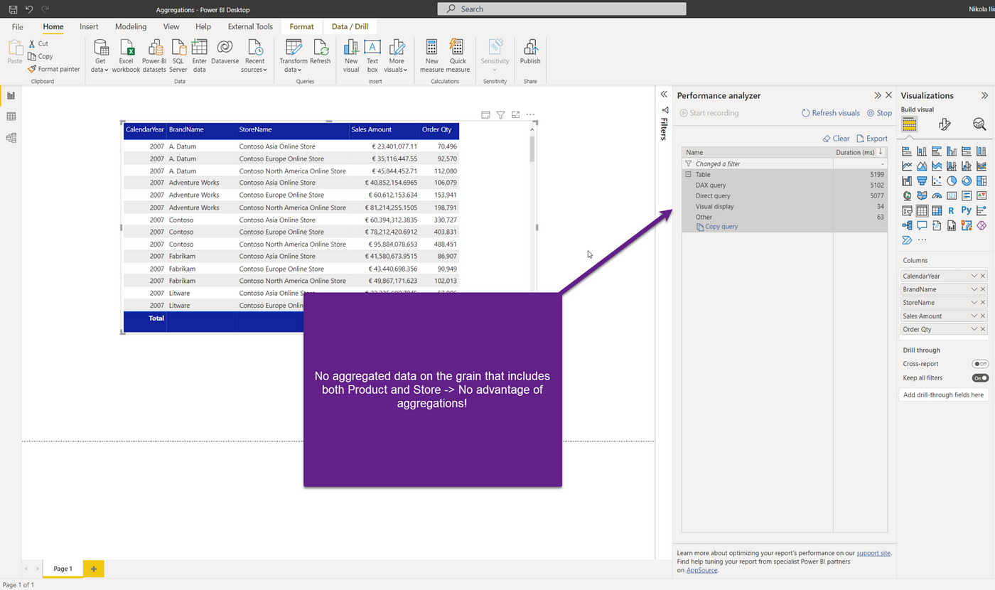
Image by author

So, in order to leverage aggregations, you need to have them defined on the exact same level of grain as the visual requires!

Aggregation Precedence

There is one more important property to understand when working with aggregations — precedence! When the Manage aggregations dialog box opens, there is an option to set the aggregation precedence:

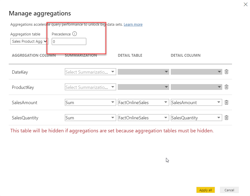
Image by author

This value “instructs” Power BI on which aggregated table to use in case the query can be satisfied from multiple different aggregations! By default, it’s set to 0, but you can change the value. The higher the number, the higher the precedence of that aggregation.

Why is this important? Well, think of a scenario where you have the main fact table with billion of rows. And, you create multiple aggregated tables on different grains:

1. Aggregated table 1: groups data on Date level — has ~ 2000 rows (5 years of dates)
2. Aggregated table 2: groups data on Date & Product level — has ~ 100.000 rows (5 years of dates x 50 products)
3. Aggregated table 3: groups data on Date, Product & Store level — has ~ 5.000.000 rows (100.000 from the previous grain x 50 stores)

Now, let’s say that the report visual displays aggregated data on the date level only. What do you think: is it better to scan Table 1 (2.000 rows) or Table 3 (5 million rows)? I believe you know the answer:) In theory, the query can be satisfied from both tables, so why rely on the arbitrary choice of Power BI?!

Instead, when you’re creating multiple aggregated tables, with different levels of granularity, make sure to set the precedence value in a way that tables with lower granularity get priority!

Conclusion

Aggregations are one of the most powerful features in Power BI, especially in scenarios with large datasets! Despite the fact that both composite models feature and aggregations can be used independently of each other, these two are usually used in synergy, to provide the most optimal balance between the performance and having all the details of the data available!

Thanks for reading!

Subscribe and don’t miss any story on Medium!