I’m a self-taught designer.1 This has its upsides: I learn at my own pace (in my case, slowly over decades and counting), I design my own curriculum, and I don’t have to do any homework or pass any tests. But it also has a serious downside: because I don’t have to learn anything, I skip the things that intimidate me. That’s why, for years and years, I’ve avoided learning much of anything about color.

But recently I picked up a pet project that forced me to fill in the gaps in my own knowledge. In the course of trying to solve a seemingly simple problem, I got a crash course in the fundamentals of color. It was (sorry, I have to get this out of my system) eye-opening.

I thought it might be worthwhile to recap my journey so far, not just to share an interesting result to a common challenge in data visualization, but also to help any other learners who have been shy about color.

The problem

Stripe’s dashboards use graphs to visualize data. While the color palettes we use are certainly passable, the team is always trying to improve them. A colleague was working on creating updated color palettes, and we discussed the challenges he was working through. The problem boiled down to this: how do I pick nice-looking colors that cover a broad set of use cases for categorical data while meeting accessibility goals?

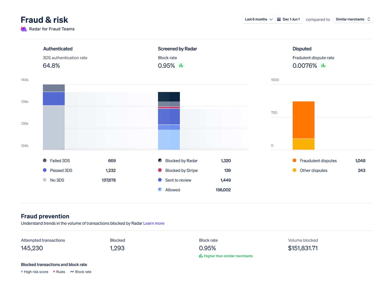
An example of Stripe’s dashboard graphs showing categorical data

The domain of this problem is categorical data — data that can be compared by grouping it into two or more sets. In Stripe’s case, we’re often comparing payments from different sources, comparing the volume of payments between multiple time periods, or breaking down revenue by product.

The criteria for success are threefold:

1. The colors should look nice. In my case, they need to be similar to Stripe’s brand colors.
2. The colors should cover a broad set of use cases. In short, I need lots of colors in case I have lots of categories.
3. The colors should meet accessibility goals. WCAG 2.2 dictates that non-text elements like chart bars or lines should have a color contrast ratio of at least 3:1 with adjacent colors.

Put this way, the problem doesn’t seem so daunting. Surely, I thought, a smart person has already solved these problems.

Prior art

There are, in fact, many ways to pick good colors for data visualizations. For example:

• Viridis is a sequential palette designed by Stéfan van der Walt and Nathaniel Smith.
• ColorBrewer is a tool and set of color palettes created by Cynthia Brewer.
• Colorgorical is a tool for selecting visually distinct colors created by Connor Gramazio with advisement from David Laidlaw and Karen Schloss.
• Companies like Adobe and IBM have documented the color palettes they use in their design systems for data visualization.

Why none of these solutions work for me

While most of the above palettes would serve as a good starting point, each has tradeoffs as an out-of-the-box solution. Using the ColorBrewer schemes sacrifices accessibility and applicability; using any of them fails to get to the harmony I want with Stripe’s brand colors.

There are many, many other approaches and palettes to try. As I looked through the research and material, I had a sinking feeling that I’d need to settle for something that wasn’t optimal.

That conclusion turned out to be a breakthrough.

Optimizing

One night, I was watching a YouTube video called “Algorithmic Redistricting: Elections made-to-order.” My YouTube recommendation algorithm is very weird and finds things like this for me; I am also very weird and like watching other people program algorithms.

In the video, Brian Haidet describes a process he used to draw different election maps. The algorithm could draw unfair maps that looked normal because Haidet used something called simulated annealing.

The name stuck in my head because it sounded cool. Googling it later, I realized simulated annealing might help me find a color palette because it works well on problems with the following qualities:

• Lots of possible solutions. I mean LOTS. One of the reasons why picking a set of colors is hard is because there are so many possible colors: a typical computer monitor in 2022 can display 16,777,216 distinct colors. That means a color palette of just three colors has 4.7 sextillion possibilities.2
• Multiple competing success criteria. Just as Haidet’s maps had to be both unfair and normal-looking, my ideal color palettes had to be Stripe-y, accessible, and broadly applicable.
• Room for error. I’m not designing a space suit; if my palette isn’t perfect, nobody is going to die.

Simulated annealing is a very complex algorithm that I will now try to explain to the best of my (admittedly limited) abilities.

How simulated annealing works

Simulated annealing is named after a process called annealing. Annealing involves getting a piece of metal white-hot, then carefully cooling it down. Metalsmiths use annealing to strengthen metals.

Here’s how it works:

1. Annealing starts with a weak piece of metal. In such a piece, the metal’s atoms are spread unevenly: Some atoms are close enough to share magnetic bonds, but others are too far apart to bond. The gaps that are left lead to microscopic deformities and cracks, weakening the metal.
2. When the weak metal is heated, the energy of heat breaks the bonds between atoms, and the atoms start to move around at random. Without the magnetic bonds between atoms, the metal is even weaker than before, making it easy to bend and reshape if needed; when the metal is glowing hot, its atoms are moving freely, spreading out evenly over time.
3. Next, the metal is placed in a special container to slowly cool. As the metal cools, the energy from heat decreases, and gradually, the atoms slow down enough to form magnetic bonds again. Because they’re more evenly spaced now, the atoms are more likely to share magnetic bonds with all their neighbors.
4. When fully cooled, the evenly-spaced atoms have many more bonds than they did before. This means there are far fewer imperfections; the metal is much stronger as a result.3

Simulated annealing is an optimization algorithm that operates on a set of data instead of a piece of metal. It follows a process similar to metallurgical annealing:

1. Simulating annealing starts with data that is in an unoptimized state.
2. The algorithm begins by making a new version of the data, changing elements at random. Changing the data is like adding heat, resulting in random variations of the data. The algorithm scores both the original and the changed data according to desired criteria, then makes a choice: keep the current state or go back to the previous one? Strangely, the algorithm doesn’t always pick the version with the better score. At first, the algorithm is “hot,” meaning it picks between the two options (the current state and the randomly-changed one) with a coin toss. This means the data can become even less optimal in the first stage of the process, just as the glowing-hot metal becomes weaker and more pliable than it was to start.
3. With each new iteration, the algorithm “cools down” a little. Here, temperature is a metaphor for how likely the algorithm is to choose a better-scoring iteration of the data. With each cycle, the algorithm is more and more likely to pick mutations that are more optimized.
4. The algorithm finishes when the data settles into a highly optimized state; random changes will almost always result in a worse-scoring iteration, so the process comes to a halt.

If we have a formula for comparing how optimized two versions of our data are, why don’t we always choose the better-scoring one? This is the key to simulated annealing. Hill-climbing algorithms, ones that always pick iterations with better scores, can quickly get stuck in what are called “local maxima” or “local minima” — states which are surrounded by less optimal neighbors but aren’t as optimal as farther-away options.

More optimalLess optimal Local maximum Global maximum

So, by sometimes picking less-optimal iterations, simulated annealing can find good solutions to problems that have complicated sets of criteria, like my problem of picking color palettes.

Choosing the right evaluation score

In applying simulated annealing to any set of data, the most important ingredient is a way of grading how optimal that data is. In my case, I needed to find a way to score a set of colors according to my desired criteria. Again, those were:

• Nice-looking (i.e., Stripe-y)
• Broadly applicable
• Accessible

For each criteria, I needed to come up with an algorithm-friendly way of numerically scoring a color palette.

Nice-looking

The first criteria was one of the most challenging to translate into an algorithmic score. What does it mean for a color to be “nice-looking?” I knew that I wanted the colors to look similar to Stripe’s brand colors because I thought Stripe’s brand colors look nice; but what makes Stripe’s brand colors look nice? I quickly realized that, in the face of hundreds of years of color theory and art history, I was way out of my depth.

And so I hope you’ll forgive me for one small cop-out: instead of figuring out a way to objectively measure how nice-looking a set of colors are, I decided it’d be much easier to start with a set of colors about which a human had already decided (for whatever reason) “these look nice.” The score for how nice-looking a set of colors is would be: “how similar they are to a given subjectively-determined-by-a-human-to-look-nice color palette?.”

Only it turns out that even the question of “how similar are these two colors” is itself a very, very deep rabbit hole. There are decades of research published in hundreds of papers on the dozens of ways to measure the distance between two colors. Fortunately for me, this particular rabbit hole was mostly filled with math.

All systems of color distance rely on the fact that colors can be expressed by numbers. The simplest way to find the distance between two colors is to measure the distance between the numbers that represent the colors. For example, you might be familiar with colors expressed in RGB notation, in which the values of the red, green, and blue components are represented by a number from 0 to 255. When the components are blended together by a set of red, green, and blue LEDs, we see the resulting light as the given color.

In programming languages like CSS, rgb(255, 255, 255) is a way to express the color white — the red, green, and blue components each have the value of 255, the maximum for this notation. Pure red is rgb(255, 0, 0). One way to measure the distance between white and red is to add each component’s colors together — for white, 255 + 255 + 255 = 765, and for red, 255 + 0 + 0 = 255 — then subtract the two resulting numbers — 765 - 255 = 510.

For reasons beyond the scope of this essay, this simple measurement of distance doesn’t match the way people perceive colors4 — for example, darker colors are easier to tell apart than lighter colors, even if they have the same simple numeric difference in their RGB values. So scientists and artists have developed other ways to measure the difference between two colors, each with its own strengths and weaknesses. Some are better at matching our perception of paint on canvas, others are better at representing the ways colors look on computer monitors.

I spent a lot of time investigating these different color measurement systems. In the end, I settled on the International Commission on Illumination’s (CIE’s) ΔE* measurement.5 ΔE* is essentially a mathematical formula that measures the perceptual difference between two colors. Perceptual is the key word: The formula adjusts for some quirks in the way that we see and perceive color. It’s still somewhat subjective, but at least it’s subjective in a way that stands up to experimental scrutiny.

The ΔE* measurement between two colors ranges from zero to 100. Zero means “these colors are identical,” and 100 means “these colors are as different as possible.” For my algorithm, I wanted to minimize the ΔE* between my algorithmically selected colors and the nice-looking colors I hand-picked.

Broadly applicable

The “broadly applicable” criteria comes up most often when providing a list of colors for designers to pick from.

Colors that are very different from one another work in a wider variety of situations than colors that are from a similar family. Combining different hues and shades gives us a larger number of colors to use if we have many categories to visualize.

Colors that are equally different from one another reduce the chance that someone viewing the chart will see a relationship that doesn’t exist in the data.

To come up with a way of numerically calculating how applicable a color palette is, my friend ΔE* came in handy. The “very different” criteria can be measured by taking the average distance between all the colors in the set — this should be as high as possible. The “equally different” criteria can be measured by taking the range of the distances between all of the colors — this should be as small as possible.

Accessible

WCAG 2.2 dictates that non-text elements like chart bars or lines should have a color contrast ratio of at least 3:1 with adjacent colors.

There are lots of colors that have a 3:1 contrast ratio with 1 other color (like a white or black background). But for something like a stacked bar chart, pie chart, or a multi-line chart, it’s likely that there will be multiple elements adjacent to each other, all with their own color. Finding just three colors with a 3:1 contrast ratio to each other is extremely challenging. Anything beyond three colors is essentially impossible.

It’s important to note that WCAG is only concerned with color contrast, just one of the ways in which colors can be perceived as different. Color contrast measures the relative “brightness” of two colors; the relative brightness of colors depends highly on whether or not you have colorblindness. The way people perceive the amount of contrast between two colors varies greatly depending on the biology of their eyes and brains.

Fortunately, addressing the WCAG contrast requirement can be done without too much difficulty. Instead of finding colors that have a 3:1 contrast ratio, use a border around the colored chart elements. As long as the chart colors are of a 3:1 contrast ratio with the border color, you’re set.

For my color palettes, I wanted to go beyond the WCAG contrast requirement and find colors that work well for people with and without color blindness. Fortunately, there is (again) a deep body of published research on mathematical ways to simulate color blindness. Like our ΔE* formula earlier, there is a formula — created by Hans Brettel, Françoise Viénot, and John D. Mollon6 — for translating the color a person without color blindness sees into the (approximate) color a person with colorblindness would see.

One bonus to this formula is that it comes with variations for the different types of colorblindness. When evaluating, we can adjust the score for each type of colorblindness, depending on how common or uncommon it is (more on this in a bit).

To determine whether a color palette works well for people with colorblindness, I first translate the colors into their color blindness equivalent using the matrix math above. Then, I measure the average of the distances between the colors using the ΔE* like we did above.

Putting it all together

At this point, I had an algorithm that could optimize a set of data in a huge solution space, and quantitative measurements of each of the criteria I wanted to evaluate for. The last step was to crunch all the quantitative measurements down into a single number representing how “good” a color palette is.

The calculation that produces this single number is called the “loss function” or “cost function.” The resulting number is the “loss” or “cost” of a set of colors. It’s essentially just a measurement of how optimized the data is; the lower the loss, the better; a loss of zero means that we have the ideal solution.7

In practice, optimizers stop long before they get to zero loss. In most optimization problems, there’s no such thing as the one right answer. There are only lots of wrong answers. Our goal is to find the least wrong one.

To that end, at the very end of my loss function, all the individual criteria scores are added together. Each is given a multiplier, which allows me to dial up or down how important a value is: Multiplying the “nice-looking” score by a higher value means that the optimizing algorithm will tend to pick nice-looking palettes, even if they aren’t as accessible or versatile.

I’m calculating scores for three different types of colorblindness, each with its own multiplier. This means that the overall tradeoffs in the algorithm are in relation to how common each type of colorblindness is.

I plug the loss function into the simulated annealing algorithm and run it. On my 2016 MacBook, the algorithm ran in about three seconds. It’s far from optimized, but not too shabby considering it generates and evaluates around 16,000 color palettes.