Staggered Treatment Effect DiD count models

So I have been dealing with various staggered treatments for difference-in-difference (DiD) designs for crime data analysis on how interventions reduce crime. I’ve written about in the past mine and Jerry’s WDD estimator (Wheeler & Ratcliffe, 2018), as well as David Wilson’s ORR estimator (Wilson, 2022).

There has been quite a bit of work in econometrics recently describing how the traditional way to apply this design to staggered treatments using two-way fixed effects can be misleading, see Baker et al. (2022) for human readable overview.

The main idea is that in the scenario where you have treatment heterogeneity (TH from here on) (either over time or over units), the two-way fixed effects estimator is a weird average that can misbehave. Here are just some notes of mine though on fitting the fully saturated model, and using post-hoc contrasts (in R) to look at that TH as well as to estimate more reasonable average treatment effects.

So first, we can trick R to use glm to get my WDD estimator (or of course Wilson’s ORR estimator) for the DiD effect with count data. Here is a simple example from my prior blog post:

# R code for DiD model of count data
count <- c(50,30,60,55)
post <- c(0,1,0,1)
treat <- c(1,1,0,0)

df <- data.frame(count,post,treat)

# Wilson ORR estimate
m1 <- glm(count ~ post + treat + post*treat,data=df,family="poisson")
summary(m1)

And here is the WDD estimate using glm passing in family=poisson(link="identity"):

m2 <- glm(count ~ post + treat + post*treat,data=df,
          family=poisson(link="identity"))
summary(m2)

And we can see this is the same as my WDD in the ptools package:

library(ptools) # via https://github.com/apwheele/ptools
wdd(c(60,55),c(50,30))

Using glm will be more convenient than me scrubbing up all the correct weights, as I’ve done in the past examples (such as temporal weights and different area sizes). It is probably the case you can use different offsets in regression to accomplish similar things, but for this post just focusing on extending the WDD to varying treatment timing.

Varying Treatment Effects

So the above scenario is a simple pre/post with only one treated unit. But imagine we have two treated units and three time periods. This is very common in real life data where you roll out some intervention to more and more areas over time.

So imagine we have a set of crime data, G1 is rolled out first, so the treatment is turned on for periods One & Two, G2 is rolled out later, and so the treatment is only turned on for period Two.

Period    Control     G1     G2
Base          50      70     40
One           60      70     50
Two           70      80     50

I have intentionally created this example so the average treatment effect per period per unit is 10 crimes. So no TH. Here is the R code to show off the typical default two-way fixed effects model, where we just have a dummy variable for unit+timeperiods that are treated.

# Examples with Staggered Treatments
df <- read.table(header=TRUE,text = "
 Period    Control     G1     G2
 Base          50      70     40
 One           60      70     50
 Two           70      80     50
")

# reshape wide to long
nvars <- c("Control","G1","G2")
dfl <- reshape(df,direction="long",
               idvar="Period",
               varying=list(nvars),
               timevar="Unit")

dfl$Unit <- as.factor(dfl$Unit)
names(dfl)[3] <- 'Crimes'

# How to set up design matrix appropriately?
dfl$PostTreat <- c(0,0,0,0,1,1,0,0,1)

m1 <- glm(Crimes ~ PostTreat + Unit + Period,
          family=poisson(link="identity"),
          data=dfl)

summary(m1) # TWFE, correct point estimate

The PostTreat variable is the one we are interested in, and we can see that we have the correct -10 estimate as we expected.

OK, so lets create some treatment heterogeneity, here now G1 has no effects, and only G2 treatment works.

dfl[dfl$Unit == 2,'Crimes'] <- c(70,80,90)

m2 <- glm(Crimes ~ PostTreat + Unit + Period,
          family=poisson(link="identity"),
          data=dfl)

summary(m2) # TWFE, estimate -5.29, what?

So you may naively think that this should be something like -5 (average effect of G1 + G2), or -3.33 (G1 gets a higher weight since it is turned on for the 2 periods, whereas G2 is only turned on for 1). But nope rope, we get -5.529.

We can estimate the effects of G1 and G2 seperately though in the regression equation:

# Lets seperate out the two units effects
dfl$pt1 <- 1*(dfl$Unit == 2)*dfl$PostTreat
dfl$pt2 <- 1*(dfl$Unit == 3)*dfl$PostTreat

m3 <- glm(Crimes ~ pt1 + pt2 + Unit + Period,
          family=poisson(link="identity"),
          data=dfl)

summary(m3) # Now we get the correct estimates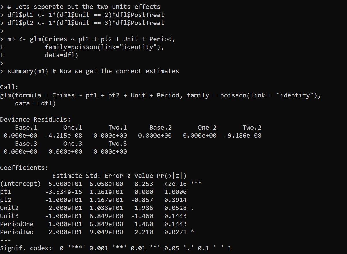

And now we can see that as expected, the effect for G2 is the pt2 coefficient, which is -10. And the effect for G1, the pt1 coefficient, is only floating point error different than 0.

To then get a cumulative crime reduction effect for all of the areas, we can use the multcomp library and the glht function and construct the correct contrast matrix. Here the G1 effect gets turned on for 2 periods, and the G2 effect is only turned on for 1 period.

library(multcomp)
cont <- matrix(c(0,2,1,0,0,0,0),1)
cumtreat <- glht(m3,cont) # correct cumulative
summary(cumtreat)

And if we want an ‘average treatment effect per unit and per period’, we just change the weights in the contrast matrix:

atreat <- glht(m3,cont/3) # correct average over 3 periods
summary(atreat)

And this gets us our -3.33 that is a more reasonable average treatment effect. Although you would almost surely just focus on that the G2 area intervention worked and the G1 area did not.

You can also fit this model alittle bit easier using R’s style formula instead of rolling your own dummy variables via the formula Crimes ~ PostTreat:Unit + Unit + Period:

But, glht does not like it when you have dropped levels in these interactions, so I don’t do this approach directly later on, but construct the model matrix and drop non-varying columns.

Next lets redo the data again, and now have time varying treatments. Now only period 2 is effective, but it is effective across both the G1 and G2 locations. Here is how I construct the model matrix, and what the resulting sets of dummy variables looks like:

# Time Varying Effects
# only period 2 has an effect

dfl[dfl$Unit == 2,'Crimes'] <- c(70,80,80)

# Some bookkeeping to make the correct model matrix
mm <- as.data.frame(model.matrix(~ -1 + PostTreat:Period + Unit + Period, dfl))
mm <- mm[,names(mm)[colSums(mm) > 0]] # dropping zero columns
names(mm) <- gsub(":","_",names(mm))  # replacing colon
mm$Crimes <- dfl$Crimes
print(mm)

Now we can go ahead and fit the model without the intercept.

# Now can fit the model
m6 <- glm(Crimes ~ . -1,
          family=poisson(link="identity"),
          data=mm)

summary(m6)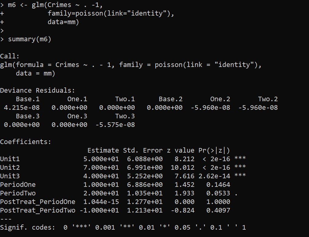

And you can see we estimate the correct effects here, PostTreat_PeriodOne has a zero estimate, and PostTreat_PeriodTwo has a -10 estimate. And now our cumulative crimes reduced estimate -20

cumtreat2 <- glht(m6,"1*PostTreat_PeriodOne + 2*PostTreat_PeriodTwo=0")
summary(cumtreat2)

And if we did the average, it would be -6.66.

Now for the finale – we can estimate the saturated model with time-and-unit varying treatment effects. Here is what the design matrix looks like, just a bunch of columns with a single 1 turned on:

# Now for the whole shebang, unit and period effects
mm2 <- as.data.frame(model.matrix(~ -1 + Unit:PostTreat:Period + Unit + Period, dfl))
mm2 <- mm2[,names(mm2)[colSums(mm2) > 0]] # dropping zero columns
names(mm2) <- gsub(":","_",names(mm2))  # replacing colon
mm2$Crimes <- dfl$Crimes
print(mm2)

And then we can fit the model the same way:

m7 <- glm(Crimes ~ . -1,
          family=poisson(link="identity"),
          data=mm2)

summary(m7) # Now we get the correct estimates

And you can see our -10 estimate for Unit2_PostTreat_PeriodTwo and Unit3_PostTreat_PeriodTwo as expected. You can probably figure out how to get the cumulative or the average treatment effects at this point:

tstr <- "Unit2_PostTreat_PeriodOne + Unit2_PostTreat_PeriodTwo + Unit3_PostTreat_PeriodTwo = 0"
cumtreat3 <- glht(m7,tstr)
summary(cumtreat3)

We can also use this same framework to get a unit and time varying estimate for Wilson’s ORR estimator, just using family=poisson with its default log link function:

m8 <- glm(Crimes ~ . -1,
          family=poisson,
          data=mm2)

summary(m8)

It probably does not make sense to do a cumulative treatment effect in this framework, but I think an average is OK:

avtreatorr <- glht(m8,
  "1/3*Unit2_PostTreat_PeriodOne + 1/3*Unit2_PostTreat_PeriodTwo + 1/3*Unit3_PostTreat_PeriodTwo = 0")
summary(avtreatorr)

So the average linear coefficient is -0.1386, and if we exponentiate that we have an IRR of 0.87, so on average when a treatment occurred in this data a 13% reduction. (But beware, I intentionally created this data so the parallel trends for the DiD analysis were linear, not logarithmic).

Note if you are wondering about robust estimators, Wilson suggests using quasipoisson, e.g. glm(Crimes ~ . -1,family="quasipoisson",data=mm2), which works just fine for this data. The quasipoisson or other robust estimators though return 0 standard errors for the saturated family=poisson(link="identity") or family=quasipoisson(link="identity").

E.g. doing

library(sandwich)
cumtreat_rob <- glht(m7,tstr,vcov=vcovHC,type="HC0")
summary(cumtreat_rob)

Or just looking at robust coefficients in general:

library(lmtest)
coeftest(m7,vcov=vcovHC,type="HC0")

Returns 0 standard errors. I am thinking with the saturated model and my WDD estimate, you get the issue with robust standard errors described in Mostly Harmless Econometrics (Angrist & Pischke, 2008), that they misbehave in small samples. So I am a bit hesitant to suggest them without more work to establish they behave the way they should in smaller samples.

References

• Angrist, J.D., & Pischke, J.S. (2008). Mostly Harmless Econometrics. Princeton University Press.
• Baker, A.C., Larcker, D.F., & Wang, C.C. (2022). How much should we trust staggered difference-in-differences estimates? Journal of Financial Economics, 144(2), 370-395.
• Wheeler, A.P., & Ratcliffe, J.H. (2018). A simple weighted displacement difference test to evaluate place based crime interventions. Crime Science, 7(1), 1-9.
• Wilson, D.B. (2022). The relative incident rate ratio effect size for count-based impact evaluations: When an odds ratio is not an odds ratio. Journal of Quantitative Criminology, 38(2), 323-341.