Portfolio Risk - Part 2: Evaluation

This is a continuation of the previous post, so I’ll be skipping some preliminary setup. This blog tries to capture tidbits of learnings from working with Gappy who is my sole mentor in my dive into modern portfolio theory. Gappy has taught at Cornell and wrote a whole book on this subject (one of the few books I go back to read over and over again).

Noone makes a good risk model in one go. It’s important to understand how to evaluate a risk model in order to iteratively improve on it with respect to those performance characteristics. Unlike a typical supervised machine learning problem, evaluating a risk model is even more involved.

Disclaimer: I’m not responsible for any hillarious losses incurred by a portfolio inspired by methodologies listed below.

Table of Contents

Structural evaluation

There are both qualitative and quantitative checks we should do to ensure the risk model is well defined and adequately captures the structure of asset returns. To do this, we’ll zoom into the loadings and the induced idiosyncratic covariance matrix.

Loadings pervasiveness & degeneracy

A factor model’s loading B can be either observable metrics of a given asset or a result of a statistical model. For an example, if we take the market cap of an asset as its loadings, we would essentially be describing the asset’s exposure to the size factor. These m loadings would be column vectors in B:

B=[||...|b1b2...bf||...|]

Loadings for a large factor model should be pervasive. This roughly means ||bi||=O(n) i.e. the norm of each loading should scale roughly linearly to the number of n assets. If there are many zeros in a particular loading, it may be trying to capture small group structure amongst the assets and is not a good candidate as a factor.

Sometimes loadings are linearly dependent (or close enough) which leads to degeneracy during regression. Using ordinary least squares, we need to invert the gram matrix of B. If there is no ridge term, we would get an error during estimation.

(BTB)−1BTr=f

The offending factors can be identified using Gram Schmidt and removed during the estimation phase. The US barra model for example has the linearly dependent factor “country” which is a linear combination of all the “industry” factors that makes up the country’s asset universe.

Idiosyncratic covariance

The idiosyncratic covariance matrix here is an ex post(measured from historical data) statistic: Ωi:=Ωr−BΩfBT where B∈Rm×f,Ωr∈Rm×m,Ωf∈Rf×f. The loadings B is often constructed statistically (e.g. using PCA or other dimensionality reduction techniques) or fundamentally (e.g. using asset characteristics like market cap). The returns and factor covariance matrices can be estimated in a few ways:

1. Using exponential weighted moving average updates of centered outer products of historical asset/factor returns to form a full rank covariance matrix.
2. Fit a multivariate GARCH model over the observed asset/factor returns to generate per-period covariance matrices.
3. Estimate a Wishart distribution from historical asset/factor returns and use the parameter Σ as a covariance estimate.

Regardless of the estimation technique, we would like to get Ωi and visualize the highly correlated clusters.

Correlation clustering

The problem of correlation clustering is NP complete, and can be framed as an graph optimization problem. Given a undirected graph G(V,E), the output of correlation clustering is C=C1,C2,…,Ck clusters where Ci=(Vi,Ei) such that Vi is a partition of the vertices, and edges are the corresponding edges that belong to all nodes in each cluster. In our case, the graph node are the n assets and the n2 edges are the correlations between assets (sometimes we use the absolute value of correlation here. For simplicity we just take the raw correlation below). The more negative the correlation of assets i and j, the less we’d like to include assets i and j in the same correlation cluster. Rigorously, define a δ function:

δ(i,j)={1if i, j are in same cluster0if i, j are in different clusters

then:

f+(C)=∑i,j:ei,j>0−ei,jδ(i,j)+∑i,j:ei,j>0ei,j(1−δ(i,j))

where the left term is the reward for putting correlated nodes in the same cluster, and the right term is the penalty for putting correlated nodes in different clusters. Similarly for anti-correlated nodes:

f−(C)=∑i,j:ei,j<0ei,jδ(i,j)+∑i,j:ei,j<0−ei,j(1−δ(i,j))

where the left term is the penalty for putting anticorrelated nodes in the same cluster, and the right term is the reward for putting anticorrelated nodes in different clusters. We would like to minimize the following:

f(C):=f+(C)+f−(C)

and the correct clustering is:

C∗=argminCf(C)

Unfortunately we cannot phrase this in a linear programming setup since membership of clusters can only be decayed to an integer linear programming problem (which is NP complete). Luckily, we have a nondeterministic 3-approximation algorithm producing ˆC, where 3-approximation is defined as:

f(ˆC)≤3f(C∗)

The procedure looks like (actual code available in a gist):

def cluster(vertices):
	v := random vertex
	c := all nodes with positive edges to v (including v)
	[c1, ..., cn] := cluster(vertices - c)
	return [c, c1, ..., cn]

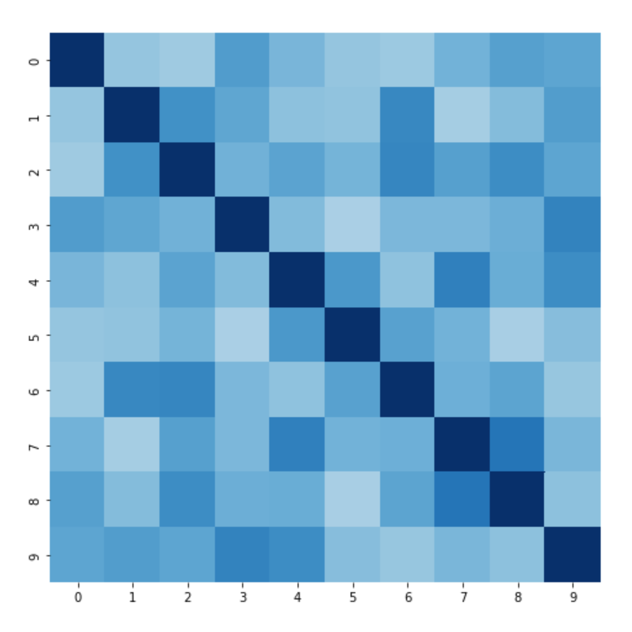
For illustration purposes, here’s a synthetic covariance matrix of 10 assets:

This is after we re-ordered the row/column axes according to clusters:

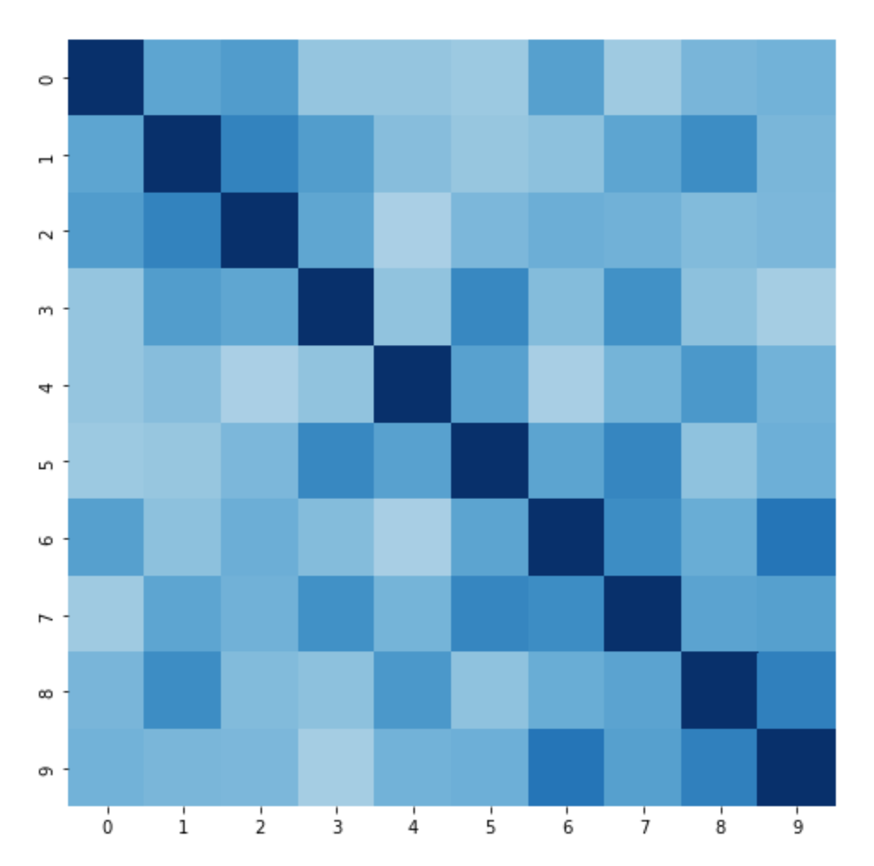
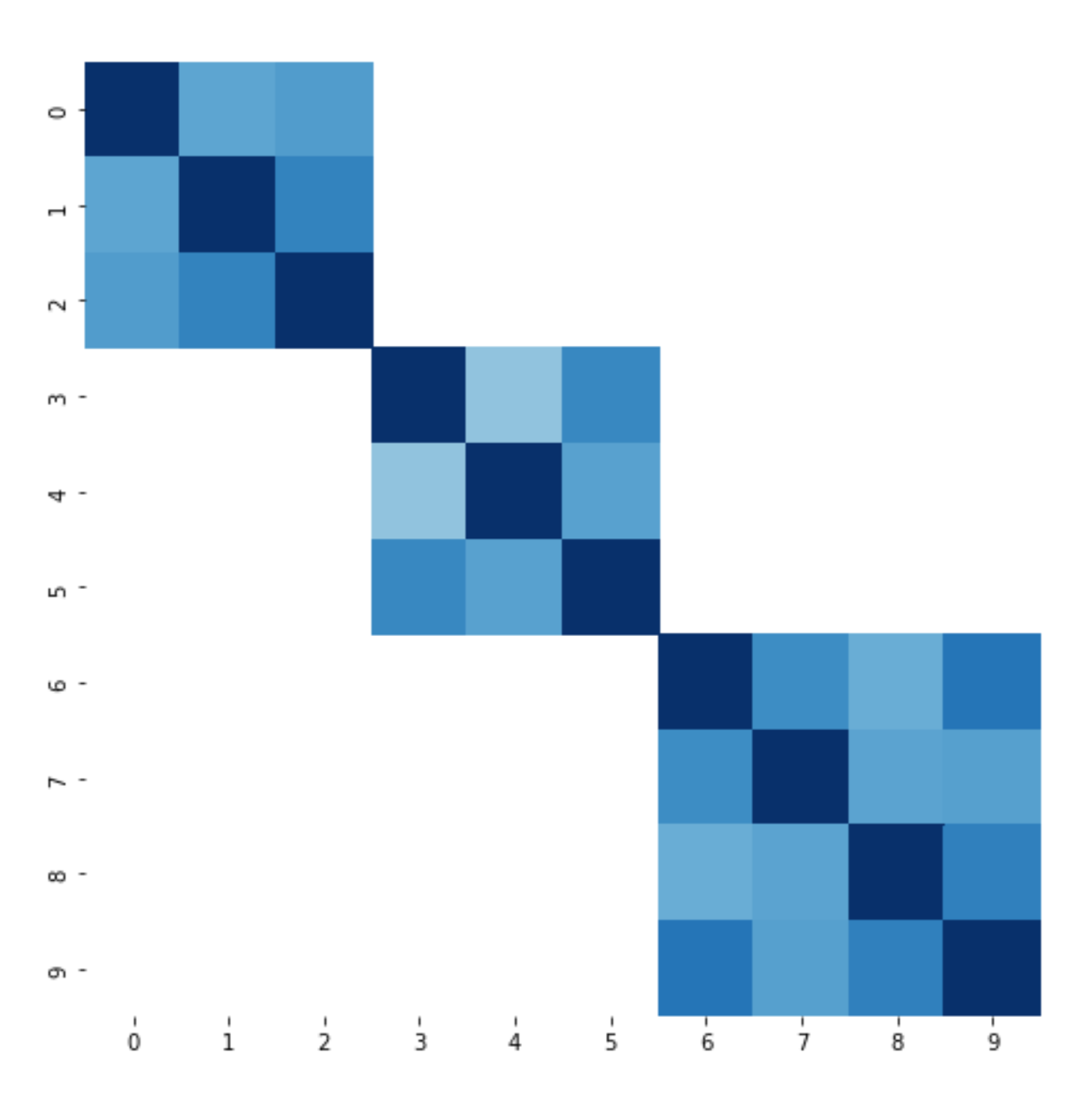
As we can see, the clustering did a pretty good job at including positive edges(darker colors is better):

… and excluding negative edges:

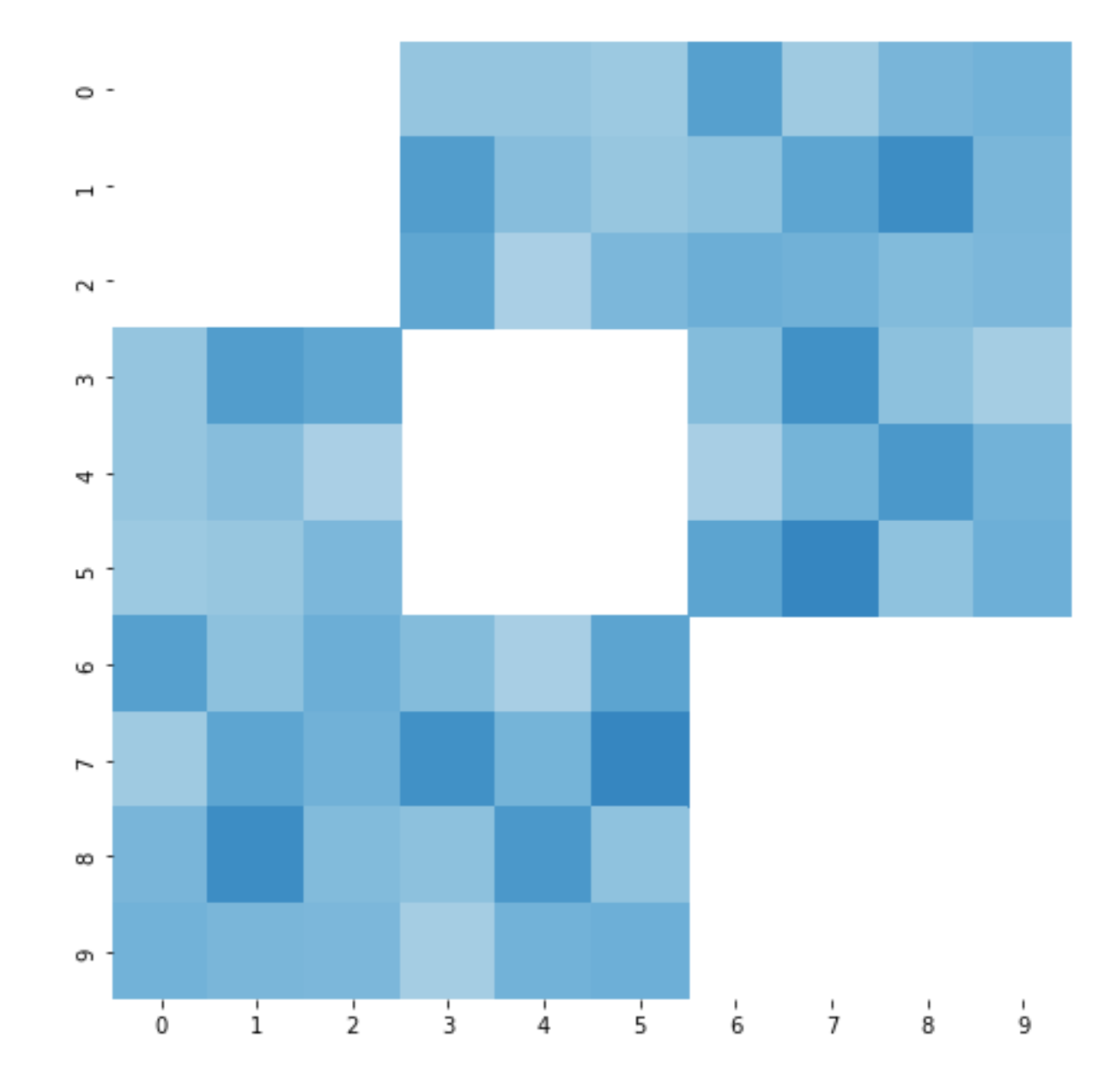
Of course, there are also other approaches to clustering that may be useful, such as hierarchical clustering using dendrograms (example visualization here). It’s always a good idea to inspect the idiosyncratic correlation matrix clusters to get an intuitive idea of the relationship between assets in your investment universe.

Microstructure

With f«m, there must be some local structure the factor model cannot accurately capture. For example, there are only a handful of major public bank stocks which have very highly correlated historical returns. Another example is the INTL vs. AMD marketshare battle - when one company gets a major data center contract for a million server-grade CPU’s, the other company loses that contract. These two stoks exhibit consistently negative correlation in less volatile market conditions. In both cases, adding a new banking factor or a microprocessor manufacturing factor for a small set of stocks would violate the pervasiveness requirement of loadings.

The astute reader may realize that there is no solution to this qualitative problem. This is inherently a problem with factor models, and the modeler should use the right tool for the job. If the investment universe only consists of tightly correlated assets with significant microstructure, maybe a factor model isn’t the right approach.

Macrostructure

Sometimes, a factor model is the right approach but we’re lacking some important factors that influence the returns of a large set of assets. This usually means there are macro correlation clusters that should be encapsulated by factors. Quantitatively, this can be found by performing PCA on the idiosyncratic covariance matrix and getting the first few largest eigenvalues. If our factor model is large & optimal, we would assume the eigenvalues to be very small. If the eigenvalues are large we can incorporate the eigenvectors as loadings or interpret the eigenvectors to be some properties about the assets(which makes the factors more tradeable).

However depending on the purpose of the risk model, this isn’t always a relevant performance characteristic to consider. For example, a risk model with very few but tradeable factors (e.g. index tracking factors) that explain the majority of the variance of a portfolio is a great hedging tool. Having very few tradeable factors means it is feasible to hedge a strategy based on the model (it would be really hard to hedge a portfolio using 100+ instruments). On the other hand, the idiosyncratic covariance matrix is bound to have lots of uncaptured macrostructure. This is often a tradeoff a portfolio manager is willing to make.

Marchenko-Pastur

Similar to asking “is there macrostructure in our idiosyncratic covariance matrix”, we can ask “does the idiosyncratic covariance matrix match our assumptions?”. We estimated our factor model such that the idiosyncratic returns are zero-centered gaussian noise. What’s the likelihood that our assumptions are correct?

In the field of random matrix theory (RMT), we’ll loosely1 define a random matrix drawn from a Wishart ensemble as a matrix X constructed from the following steps:

First create a matrix M∈Rn×m such that Mi,j∼N(μ,σ2) are independently sampled. This matches our assumptions if for each row in M we have the idiosyncratic returns for that day.

We then symmetrize the matrix by taking X:=MTMn. Assuming idiosyncratic returns have mean 0, this is the covariance matrix. The eigenvalues of a symmetric matrix are real and non-negative, so it’s a positive semidefinite matrix. The joint probability distribution of this matrix is proportional to:

p(X)∝e−12tr(X)det(X)12(n−m−1)

Two random dudes named Marchenko and Pastur were looking at the spectral density of the Wishart ensemble by asking the question “what happens to the distribution of eigenvalues of X asymptotically as n and m increase?”. As m increases, X becomes a larger square matrix with more non-negative eigenvalues. As n increases, we can use the law of large numbers to reach some convergence guarrantees(we also need n to increase so the covariance matrix is not degenerate). Under the assumption that n and m grow in some asymptotic ratio c:=m/n, they were able to find the spectral density function f(x) as:

f(x)=12πcx√(b−x)(x−a)

with support [a,b], where a,b=±(1−√c)2. The distribution looks like this with c<1:

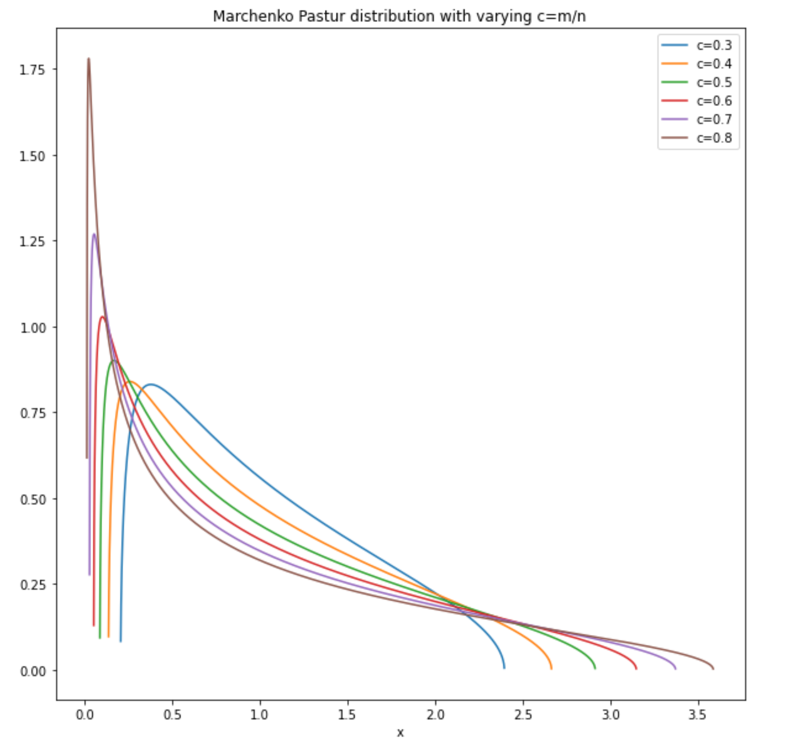
For c>1:

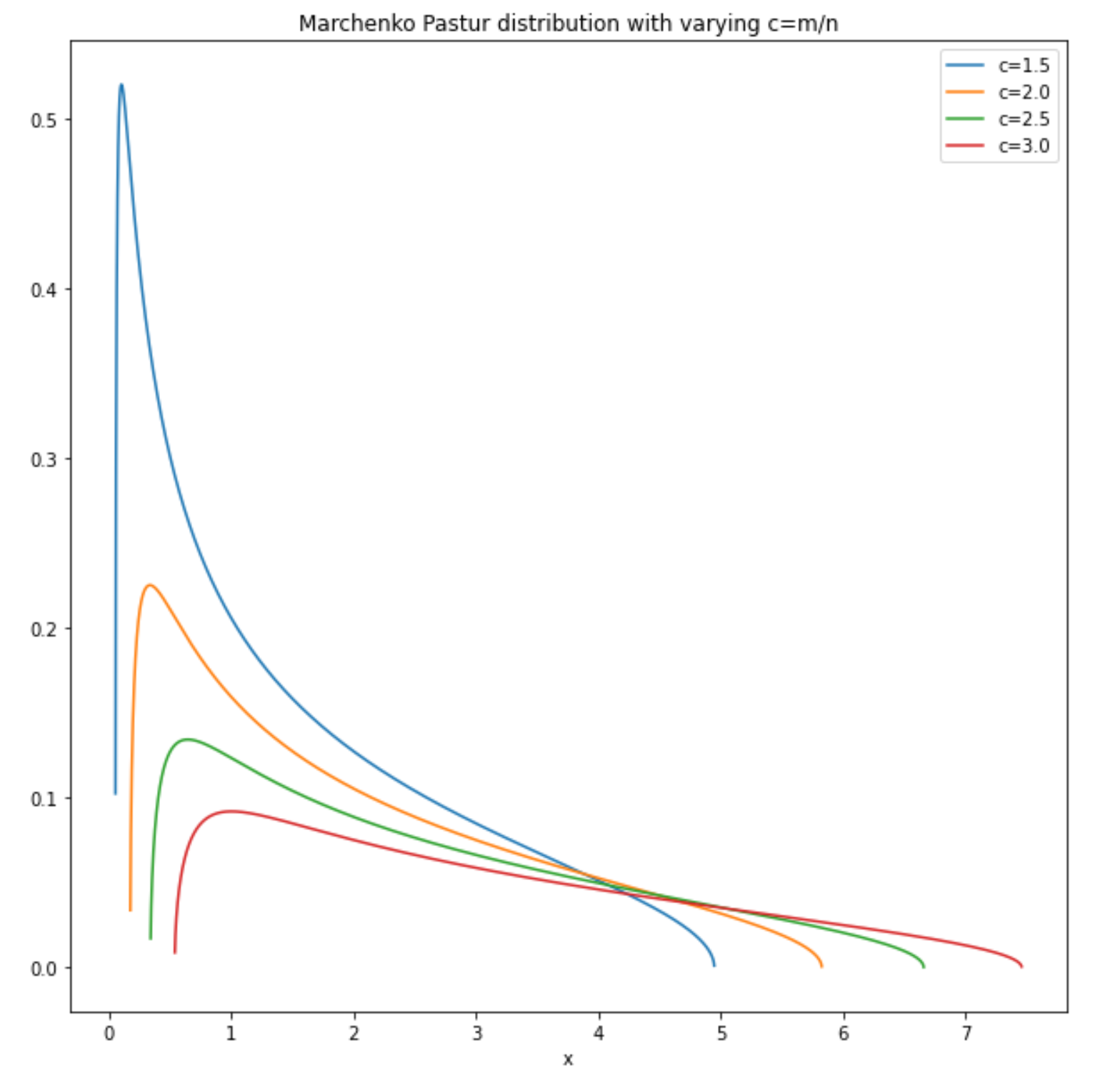
If we can derive a reasonable c either by getting a maximum likelihood estimate from our idiosyncratic covariance matrix or by an educated forecast, we can calculate the likelihood that the eigenvalues of our idiosyncratic covariance matrix is sampled from the Marchenko-Pastur distribution. The higher the likelihood, the more likely our idiosyncratic returns are gaussian random noise.

John’s sphericity test

Marchenko and Pastur have given us a useful tool to measure how likely our idiosyncratic covariance matrix belongs to a Wishart ensemble (the underlying idiosyncratic returns is gaussian noise). Another trait we’ve assumed about our idiosyncratic covariance matrix is that the off-diagonal entries should be zero as in the noise is uncorrelated. Some random dude named John came up with this statistic in the 1970’s:

U=1mtr((Ctr(C)/m)−I)2)

Here, C is our correlation matrix(which can be directly derived from Ω, our covariance matrix). Since trace is rotation invariant, the quantity inside is roughly equivalent to the squared error between the eigenvalues of a spherical distribution and the elliptical idiosyncratic covariance distribution. The score by itself has little interpretability. Comparing between two different models under the same symbol universe (for same m) allows us to understand which model has a better idiosyncratic covariance matrix - a lower score is “more diagonal” and better.

Loss functions

Loss functions is a straightforward method to quantitatively reason about the performance of a model. Loss functions output a number - if it’s high we’re sad and if it’s low we’re happy. The number usually isn’t interpretable so it is only useful when there are multiple numbers corresponding to different models to compare with.

Typical supervised learning problem often have simple loss functions. A common choice is to use the negative log-likelihood as your loss function with some regularization terms in the lagrangian. The intuition is simple - try to select an estimator from a family of function with relatively low bias and variance.

In the context of backtesting factor models, we can use loss functions to evaluate the accuracy of predicted portfolio variance. Concretely, variance loss functions are mappings of the form:

f:RT+×RT+→R

This reads “the function takes in two vectors containing positive values indexed by time and outputs a real number”. One of the positive vector arguments is the actual portfolio variance across days, and the other is the predicted portfolio variance across days. We can almost consider the actual portfolio variance as the labels of the training set. Unfortunately, we can’t observe the variance of any assets at a single point in time! Asset variance is a nonstationary, latent quantity so we don’t have any labels for our predictions! What do we do?

Proxies (ex post)

Proxies are able to give a reasonable volatility estimate to use as labels to compare against predictions. A simple volatility proxy can be computed as:

σ2=(wTr)2σ=|wTr|

The above proxy is very noisy but has less bias than some types of estimates, making this a bias-variance tradeoff problem. We now have some noisy estimates of our labels, which isn’t the most satisfying but we tread onwards.

Predictors (ex ante)

Given a factor model, we can calculate the covariance matrix using:

ˆΩ=BΩfBT+Ωi

where Ωi is a diagonal covariance matrix, B is the loadings of symbols to factors, and Ωf is the full factor covariance matrix.

Given a portfolio w∈Rm, we can predict its variance:

ˆσ2=wTˆΩw

Now that we have the two inputs to a loss function, let’s choose our functions!

MSE or mean squared error is the classic loss function everyone should know about. It’s literally just the average euclidean distance between σ2 and ˆσ2 over dates:

MSE(ˆσ2,σ2):=1T||ˆσ2−σ2||22=1T∑t(ˆσ2t−σ2t)2

The farther away our predicted portfolio variance, the higher the loss. If our prediction is exactly accurate, the loss would be 0.

One consequence of having a very noisy variance estimate is that the squared distance per time may be really different. Imagine our variance proxy outputted a total of 100thefirstday,andatotalof1,000,000 the second day. If we were to predict 1thefirstdayand999,000 the second day, the second day distance would dominate the loss function purely due to the magnitude of the proxy. In reality, we were really close to predicting the second day’s variance - it’s just harder to be exact when the magnitude is larger. To alleviate this problem, we typically use a normalized MSE:

MSE′(ˆσ2,σ2):=1T||σ2ˆσ2−1||22

which removes the noise introduced by varying magnitudes.

QLike

QLike or quasi-likelihood is an improvement on MSE for σ2 estimations. It’s defined as follows:

QLIKE(ˆσ2,σ2):=1T∑t−log(σ2t^σt2)+σ2t^σt2−1

Note the logarithmic term doesn’t allow any negative variance predictions which is great (MSE doesn’t care in comparison). When the ratio of proxy to prediction is small, the negative log term dominates the loss function. When the ratio of proxy to prediction is large, the linear term dominates the loss function. The sum of these convex functions form a convex function with a single minima at the ratio being 1.

If we set x:=σ2t^σt2 and perform a taylor expansion at x=1, we see the following:

QLIKE(x)≈0+(−1+1)(x−1)+(1)(x−1)22+o(||x3||)≈MSE′(x)

Locally, it seems like quasi likelihood is very similar to a normalized mean squared error! So what is this quasi-likelihood and why do we care?

What is Quasi-Likelihood?

Recall that in a typical linear regression, we assume E(y|x) is a linear function in x, so that:

y=βTx+ϵ

For some β. The noise around the mean is usually assumed to be i.i.d gaussian:

ϵ∼N(0,σ2)

These assumptions can be relaxed and generalized to fit other expectation functions with noise from an exponential family distribution. For example, we can perform a gamma regression with(you don’t need to know this):

y=eβTx+ϵ

which is better modeling choice when y≥0. Denoting E(y|x)=μ, the noise from a gamma regression is assumed to be:

ϵ∼Γ(0,μβ2)

However, when the underlying distribution is unknown (e.g. the variance of our portfolio), how can we assign a likelihood function? One way to get around this is to construct a quasi-likelihood model, which not only assumes y=h(βTx)+ϵ for some h, but also ϵ is a zero-mean distribution with variance as a function of the mean of y|x:

V(ϵ)=ϕV(μ)

Here ϕ is a hyperparameter and V is a function we construct. Note how previously we specified the exact distribution of ϵ, but now we only characterize ϵ by its first and second moments? This is because we don’t know the underlying distribution, and that’s where the “quasi” part comes from.

Since we don’t have a likelihood(or log-likelihood) function, we’re gonna have to make one. The log-likelihood function is an integral of the score function, which has the following requirements:

E(S(μ))=0V(S(μ))=−E(∂S(μ)∂μ)

We define a quasi-score function as:

S(μ)=y−μϕV(μ)

which has a zero mean:

E(S(μ))=∫y−μϕV(μ)p(y)dy=∫yp(y)dy−μϕV(μ)=μ−μϕV(μ)=0

The variance is:

V(S(μ))=E(S(μ)2)−E(S(μ))2=∫(y−μϕV(μ))2p(y)dy−02=∫y2p(y)dy−2μ2+μ2(ϕV(μ))2=E(y2)−E(y)2V(y)2=1V(y)

And it satisfies the constraints of a score function:

−E(∂S(μ)∂μ)=E((μ−y)∂V(μ)∂μ−V(μ)ϕV(μ)2)=1V(y)

Given some choices of V(μ), we would get appropriate quasi log-likelihoods by integration. For example, if we chose V(μ)=1, we would get a normal distribution with quasi-likelihood equal to:

logL(μ,y)=−(y−μ)22

The quasi log-likelihood we chose is consistent with the construction above if we set ϕ=1 and V(μ)=μy, and we were able to create it without knowing what the underlying distribution is, which may not be a member of the exponential family. For more information on the choice of V, refer to the paper “Volatility Forecast Comparison using Imperfect Volatility Proxies” by A.J. Patton.

Test portfolios

Now that we’ve defined some loss functions, we need to choose appropriate test portfolios to estimate the variance. There are tons of different test portfolios that may be useful, but we’ll outline a few here.

Historical strategy portfolios

If you’re backtesting your factor model, the first thing that comes to mind should be to evaluate it on your historical portfolios! Arguably, there is no cleaner, practical dataset to evaluate on than your own strategies, which you’ve either made or lost tons of money on. You know what the variance of your PnL looks like better than anyone else, and that serves as an additional heuristic to measure the performance of your portfolios aside from the noisy variance proxy.

Benchmark portfolios

Benchmarks portfolios track the weights of constituents of a large index. For example, we can have a benchmark portfolio tracking S&P500 by securitizing any S&P500 ETF like IVV. A comprehensive factor model should be able to predict the benchmark portfolios variance accurately. Surprisingly, we have a pretty good proxy for the S&P500 volatility - VIX! If our predicted volatility is way off from the historical VIX values, there’s a good chance our factor model performs really badly.

Benchmarks in general span a large set of assets so we expect the variance proxies to be less noisy, which helps us interpret the loss function metrics.

Minimum variance portfolios

Given a risk model, we can construct a portfolio that is the result of an optimization problem:

maxweTws.t.wTΩw≤1

where e is the vector of all 1’s. This is the portfolio corresponding to the largest notional holding possible with unit portfolio variance. If we focused on the set of solutions such that wTΩw=1, this allocation gives us the maximum capital investment(but not returns!) fixed to a variance. This portfolio should stay relatively stable over time with relatively low variance (the model should predict unit variance). If the variance proxy associated with this portfolio is very large, it means the estimated Ω is not stable for e.g. mean variance optimization.

Factor mimicking portfolios

A factor mimicking portfolio is a portfolio which gives unit exposure to a single factor and zero exposure to everything else. When we estimate the factor returns (covered in previous post) in the case of weighted least squares:

ˆf=(BTWB)−1BTWr=PTr

We get an intermediate quantity P∈Rn×f:

P=[||...|p1p2...pf||...|]

When we interpret individual stacked pi as portfolios in P and try to calculate the factor exposures:

BTP=BT[(BTWB)−1BTW]T=(BTWB)(BTWB)−1=I

We see that for pi we have unit exposure to the i-th factor and zero exposure to everything else! If we are interested in the variance of a particular factor tracking portfolio (e.g. it has a positive expected return), we would use it in the loss function and see how well the model can predict the portfolio’s variance.

Hedged portfolios

Given some arbitrary portfolio, we can decompose the holdings:

w=wf+wiwf∈span(P)wTiB=0wf⊥wi

In other words, a portfolio can be decomposed to one with zero factor exposure, and another that can be constructed by some linear combination of factor mimicking portfolios. A portfolio with zero exposures is one that is hedged to the entire factor model. Calculating this is easy if we already have P.

It is important to note that although the hedged portfolio has zero factor exposure, the risk model will still predict non-zero variance due to the diagonal Ωi idiosyncratic variance term in ˆΩ=BΩfBT+Ωi. Regardless, if the variance proxy of a hedged portfolio is large it means the factor model is unable to express all risk factors and cannot hedge a portfolio appropriately.

Portfolio Statistic: Turnover

Aside from using the portfolio to compare predicted variance and variance proxies, there are other considerations when it comes to evaluating a risk model. The turnover of a portfolio is defined as:

turnover(w0,...,wT)=T∑t||wt−1∘rt−1−wt||22

Intuitively, the above expression gives us a measurement of how much a portfolio “moves” over time. In an ideal world, we’d like a portfolio that which moves minimally but still makes a boatload of money. Unfortunately we live in a society, so that means the turnover and alpha potential of the portfolio are often at odds with each other. Large turnover doesn’t only mean more work - the market impact of moving large amounts of capital is nontrivial. If we had to suddenly purchase 1 million shares of GOOG under a minute, we would crash through the order book and get filled at very suboptimal prices as well as shifting GOOG’s price up significantly.

So suppose we’ve calculated the optimal mean-variance portfolio for a given factor model - we would love to trade with it if it makes us a ton of money with relatively low risk. We should first backtest the turnover statistic of the mean-variance portfolio to see if it’s actually something we can feasibly trade. If the fees of moving from the optimal portfolio at time T to T+1 is too high, we can’t realize any profit.

Conclusion

Model evaluation is a really hard problem with no clear answers. It requires the porfolio manager to make active tradeoffs and a solid investment thesis for the corresponding evaluation suite to be useful. We looked at the construction of the factor model, and how well behaved the loadings are. We took a deep dive into the idiosyncratic covariance matrix and whether residual structures break our modelling assumptions. We discussed different loss functions with different theoretical motivations, and how we can use a variety of test portfolios to plug backtested variance estimates to comparatively evaluate our models. There are a lot of other considerations not listed in this blog, but I hope this serves as a brief introduction to evaluating your models!