Mathematics of Artificial Intelligence: The learning problem in neural networks

2. Learning problem

We can express the learning problem as finding a function that causes some functional to assume an extreme value. This functional, or loss index, defines the task the neural network is required to do and provides a measure of the quality of the representation that the network needs to learn. The choice of a suitable loss index depends on the particular application.

Here is the activity diagram.

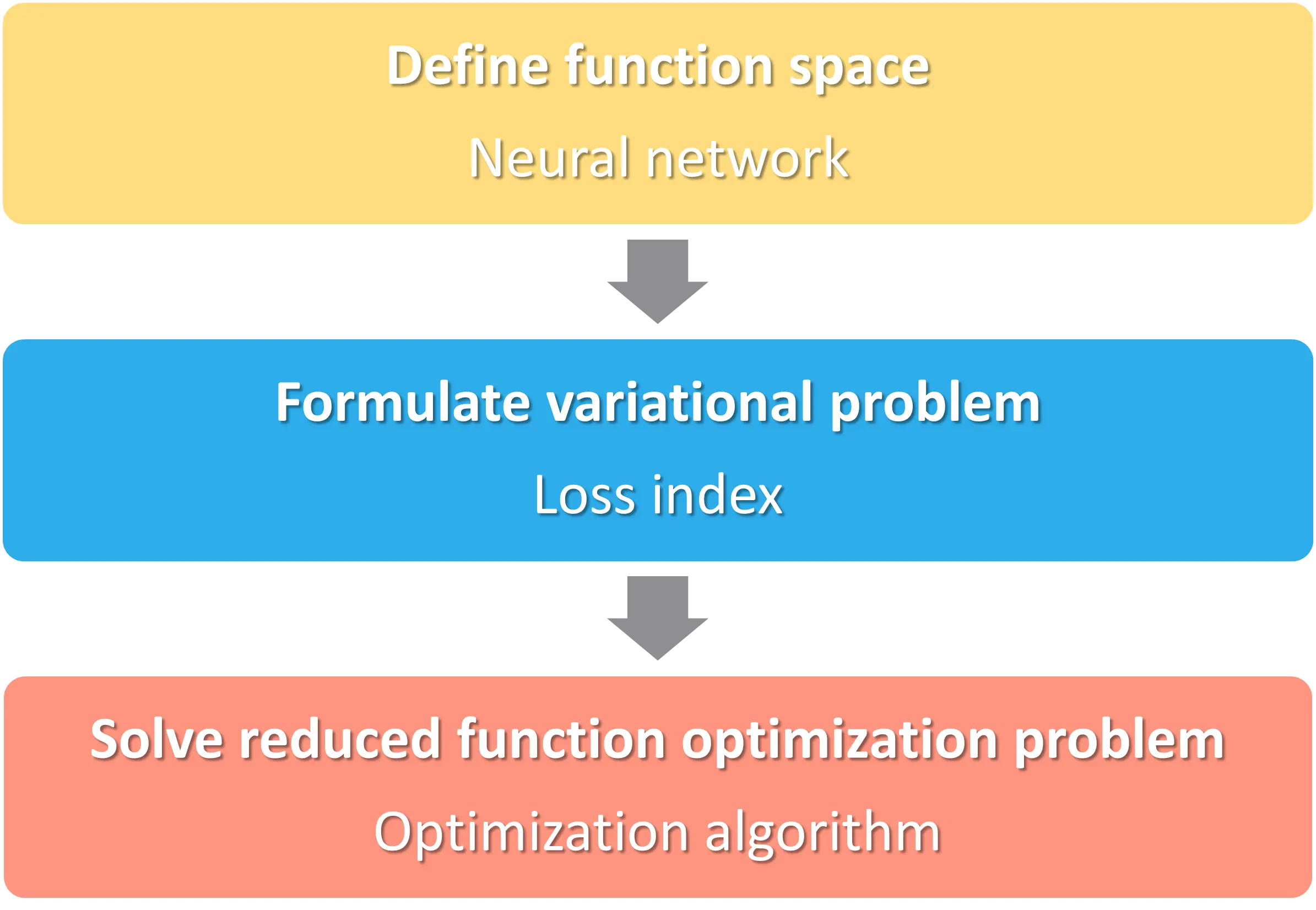
We will explain each of the steps one by one.

2.1. Neural network

A neural network spans a function space, which we will call VV. It is the space of all the functions that the neural network can produce. y:X⊂Rn→Y⊂Rmx↦y(x;θ)y:X⊂Rn→Y⊂Rmx↦y(x;θ) This structure contains a set of parameters. The training strategy will then adjust the parameters to perform specific tasks. Each function depends on a vector of free parameters θθ. The dimension of VV is the number of parameters in the neural network.

For example, here, we have a neural network. It has a hidden layer with a hyperbolic tangent activation function and an output layer with a linear activation function. The dimension of the function space is 7, the number of parameters in this neural network.

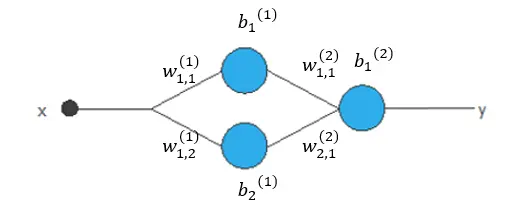
The elements of the function space are of the following form. y(x;θ)=b(2)1+w(2)1,1tanh(b(1)1+w(1)1,1x)+w(2)2,1tanh(b(1)2+w(1)1,2x)y(x;θ)=b1(2)+w1,1(2)tanh(b1(1)+w1,1(1)x)+w2,1(2)tanh(b2(1)+w1,2(1)x)

Here we have different examples of elements of the function space.

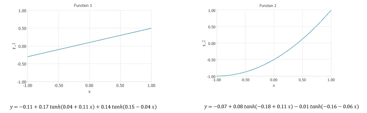
They both have the same structure but different values for the parameters.

2.2. Loss index

The loss index is a functional that defines the task for the neural network and provides a measure of quality. The choice of the functional depends on the application of the neural network. Some examples are the mean squared error or the cross-entropy error. In both these cases, we have a dataset with kk points (xi,yi)(xi,yi), and we are looking for a function y(x,θ)y(x,θ) that will fit them.

• Mean squared error: E[y(x;θ)]=1k∑ki=1(y(xi;θ)−yi)2E[y(x;θ)]=1k∑i=1k(y(xi;θ)−yi)2
• Cross-entropy error: E[y(x;θ)]=−1k∑ki=1y(xi;θ)log(yi)E[y(x;θ)]=−1k∑i=1ky(xi;θ)log(yi)

We formulate the variational problem, which is the learning task of the neural network. We look for the function y∗(x;θ∗)∈Vy∗(x;θ∗)∈V for which the functional F[y(x;θ)]F[y(x;θ)] gives a minimum value. In general, we approximate the solution with direct methods.

Let's see an example of a variational problem. Consider the function space of the previous neural network. Find the element y∗(x;θ)y∗(x;θ) such that the mean squared error functional, MSEMSE, is minimized. We have a series of points, and we are looking for a function that will fit them.

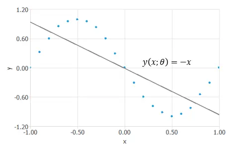
We have taken a random function y(x;θ)=−xy(x;θ)=−x for now, the functional MSE[y(x;θ)]=1.226MSE[y(x;θ)]=1.226 is not minimized yet. Next, we will study a method to solve this problem.

2.3. Optimization algorithm

The objective functional FF has an objective function ff associated. f:Θ⊂Rd→Rθ↦f(θ)f:Θ⊂Rd→Rθ↦f(θ)

We can reduce the variational problem to a function optimization problem. We aim to find the vector of free parameters θ∗∈Θθ∗∈Θ that will make f(θ)f(θ) have its minimum value. With it, the objective functional achieves its minimum.

The optimization algorithm will solve the reduced function optimization problem. There are many methods for the optimization process, such as the Quasi-Newton method or the gradient descent.

Let's continue the example from before. We have the same set of points, and we are looking for a function that will fit them. We have reduced the variational problem to a function optimization problem. To solve the function optimization problem, the optimization algorithm search for a vector θ∗θ∗ that minimizes the mean squared error function.

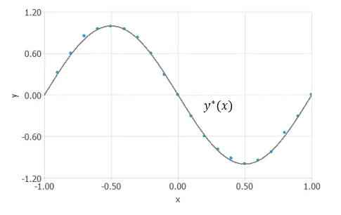
After finding this vector θ∗=(−1.16,−1.72,0.03,2.14,−1.67,−1.72,1.24)θ∗=(−1.16,−1.72,0.03,2.14,−1.67,−1.72,1.24), for which mse(θ∗)=0.007mse(θ∗)=0.007, we obtain the function y∗(x;θ∗)=−1.16−1.72tanh(0.03+2.14x)−1.67tanh(−1.72+1.24x)y∗(x;θ∗)=−1.16−1.72tanh⁡(0.03+2.14x)−1.67tanh(−1.72+1.24x) that minimizes the functional. This is the solution to the problem.