复杂网络社区发现算法python实战准备.

1 要安装的包

# 不要单独安装networkx和community ，会导致Graph没有best_parition属性
# 安装与networkx 2.x 版本对应的python-louvain(它内部包含了community)
pip install -U git+https://github.com/taynaud/python-louvain.git@networkx2
# 安装 networkx,理论上应该默认安装最新版版的 2.4
pip install networkx
# 如果上述安装之后，'Graph' object has no attribute 'edges_iter'
#需要卸载networkx 2.x版本，只能使用1.x版本。注意networkx1.x版本的函数API 不一样，
pip install  networkx==1.9.1

2 数据和参考资料

3 测试代码

我们下载使用 astro-gh数据集。

import community
from community import community_louvain
data = "./data/astro-ph/astro-ph.gml"
Graph=nx.read_gml(data)
# network2.x的图划分
part = community_louvain.best_partition(Graph)
# network1.x的图划分
part =community.best_partition(Graph)

测试代码2

import community
import networkx as nx
import matplotlib.pyplot as plt

#better with karate_graph() as defined in networkx example.
#erdos renyi don't have true community structure
#G = nx.erdos_renyi_graph(30, 0.05)
data = "./data/astro-ph/astro-ph.gml"
G=nx.read_gml(data)

#first compute the best partition
partition = community.best_partition(G)
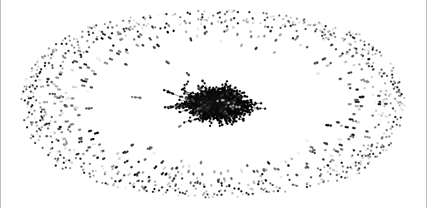
#drawing
size = float(len(set(partition.values())))
pos = nx.spring_layout(G)
count = 0.
for com in set(partition.values()) :
    count = count + 1.
    list_nodes = [nodes for nodes in partition.keys()
                                if partition[nodes] == com]
    nx.draw_networkx_nodes(G, pos, list_nodes, node_size = 20,
                                node_color = str(count / size))
nx.draw_networkx_edges(G, pos, alpha=0.5)
plt.show()

运行时间有点长，大概需要10分钟，效果如下

4 相关API

4.1 community

community API 函数比较少，主要是从网络中划分社区，而社区划分算法又只有一个默认实现。网络部分由另外一个包networkx实现。

• community.best_partition(graph, partition=None, weight='weight', resolution=1.0, randomize=None, random_state=None):使用Louvain heuristices方法划分的获得最高模块度的社区发现算法。

  • graph:networkx.Graph:需要划分的网络图。一般由直接读取的数据得到networkx.read_gml(data)
  • partition:dict, optional:里面是词典形式的数据，k为节点id，value为节点的标签。算法将以此为基础开始运算得到新的划分。
  • weight:str, optional:字符串形式的权重。作为权重的运算
  • resolution:double, optional: 改变社区的规模尺寸，默认为1.描述的是论文Laplacian Dynamics and Multiscale Modular Structure in Networks中所说的规模。
  • randomize:boolean, optional: 是否随机节点和社区的评估顺序，来获得不同的划分结果
  • random_state:int,optional:上面随机数的随机种子
  • 返回结果：新的词典形式的划分结果，key为节点id或名字，value为新的所属社区id(从0开始增长)

• community.generate_dendrogram(graph, part_init=None, weight='weight', resolution=1.0, randomize=None, random_state=None):以层次图的形式划分社区。树状图中每一层都是图中节点的一个划分。第0层为第一个划分，包含了最小的社区，最佳社区长度是树状图层次减去1，层次越高社区规模越大。

  • graph:networkx.Graph；需要划分的网络图
  • part_init:dict, optional: 算法起始社区划分，词典形式，key为节点，value为节点对应的社区
  • 其他参数与上面一样

import community
from community import community_louvain
import networkx as nx

G=nx.erdos_renyi_graph(50, 0.1)
dendo =community_louvain.generate_dendrogram(G)
for level in range(len(dendo) - 1) :
     print("partition at level", level,"is", community_louvain.partition_at_level(dendo, level))

partition at level 0 is {0: 0, 1: 1, 2: 2, 3: 3, 4: 4, 5: 5, 6: 5, 7: 6, 8: 7, 9: 3, 10: 8, 11: 5, 12: 9, 13: 10, 14: 11, 15: 12, 16: 10, 17: 11, 18: 3, 19: 11, 20: 8, 21: 10, 22: 13, 23: 7, 24: 6, 25: 14, 26: 13, 27: 2, 28: 0, 29: 13, 30: 13, 31: 5, 32: 9, 33: 6, 34: 7, 35: 15, 36: 14, 37: 10, 38: 11, 39: 2, 40: 13, 41: 15, 42: 12, 43: 3, 44: 1, 45: 0, 46: 4, 47: 12, 48: 16, 49: 16}
partition at level 1 is {0: 0, 1: 1, 2: 2, 3: 1, 4: 3, 5: 3, 6: 3, 7: 2, 8: 4, 9: 1, 10: 4, 11: 3, 12: 0, 13: 2, 14: 3, 15: 2, 16: 2, 17: 3, 18: 1, 19: 3, 20: 4, 21: 2, 22: 5, 23: 4, 24: 2, 25: 1, 26: 5, 27: 2, 28: 0, 29: 5, 30: 5, 31: 3, 32: 0, 33: 2, 34: 4, 35: 1, 36: 1, 37: 2, 38: 3, 39: 2, 40: 5, 41: 1, 42: 2, 43: 1, 44: 1, 45: 0, 46: 3, 47: 2, 48: 5, 49: 5}

• community.partition_at_level(dendrogram, level):返回指定层次的社区划分结果。使用示例如上代码。

• community.induced_graph(partition, graph, weight='weight'):产生社区聚合图，在社区之间产生一条带权重w的边，如果社区内边的总权重为w的话。

  • 其他参数跟上面一样
  • 返回值:一个新的图，其中节点为划分。

4.2 networkx

networkx 包括网络(图)的构建，添加/删除节点、边等。使用networkx构建网络图时，节点可以是任意可哈希的对象，边可以与任意对象关联。

• 构建网络图: G=networkx.Grapgh()即可构建一个空的网络图。网络是由节点和边组成的集合。
• 节点
  • 添加一个节点: G.add_node(1)
  • 添加节点列表：G.add_nodes_from([2, 3])
  • 使用包含节点的迭代器添加节点：H=networkx.path_graph(10),G.add_nodes_from(H)，此时的图H包含了一些节点，但是被视为新的节点，也可以用G.add_node(H)的方式将H作为一个节点来添加。
  • 节点删除。Graph.remove_node()删除一个节点，Graph.remove_nodes_from()删除多个节点
• 边:如果边已经存在，再次添加不会报错。
  • 可以一次添加一条边。G.add_edge(1,2)
  • 也可以一次添加多条边。边列表添加，G.add_edges_from([(1, 2), (1, 3)])。也可以使用边迭代器G.add_edges_from(H.edges)
  • 边删除。Graph.remove_edge(1,3)删除一条边，Graph.remove_edges_from()删除多条边
• 图的统计属性。我们可以查看的属性有G.nodes,G.edges,G.adj,G.degree(都是集合形式存放)。效果如下

list(G.nodes)
[1, 2, 3, 'spam', 's', 'p', 'a', 'm']
list(G.edges)
[(1, 2), (1, 3), (3, 'm')]
list(G.adj[1]) # or list(G.neighbors(1))
[2, 3]
G.degree[1] # the number of edges incident to 1
2

• 图的子集的统计属性。上面的四种属性都接收参数以指定特定的节点或边或节点子集。

G.edges([2, 'm'])
EdgeDataView([(2, 1), ('m', 3)])
G.degree([2, 3])
DegreeView({2: 1, 3: 2})

• 其他方式得到节点邻居。比如Graph[1]就可以得到节点1的所有邻居，Graph[1][2]得到节点1和2之间的边的属性。甚至可以修改属性，Graph[1][2]['color']=""blue等同于Graph.edges[1,2]['color']="blue"。
• 使用G.adjacency()或G.adj.items()即可访问所有(节点,邻居)对。注意，如果是无向图，每条边可能会出现两次。

FG = nx.Graph()
FG.add_weighted_edges_from([(1, 2, 0.125), (1, 3, 0.75), (2, 4, 1.2), (3, 4, 0.375)])
for n, nbrs in FG.adj.items():
    for nbr, eattr in nbrs.items():
        wt = eattr['weight']
        if wt < 0.5: print('(%d, %d, %.3f)' % (n, nbr, wt))

(1, 2, 0.125)
(2, 1, 0.125)
(3, 4, 0.375)
(4, 3, 0.375)

• 给图，节点，边添加属性，权重、标签、颜色等，可以是任意Python对象
  • 给图加/修改属性。networkx.Graph(day="Friday"),修改G.graph['day'] = "Monday"
  • 节点属性。 add_node(),add_nodes_from(),G.nodes
  • 边属性。使用add_edge()和add_edges_from()

# 节点属性添加和修改
>>> G.add_node(1, time='5pm')
>>> G.add_nodes_from([3], time='2pm')
>>> G.nodes[1]
{'time': '5pm'}
>>> G.nodes[1]['room'] = 714
>>> G.nodes.data()
NodeDataView({1: {'time': '5pm', 'room': 714}, 3: {'time': '2pm'}})
# 边属性修改/添加
>>> G.add_edge(1, 2, weight=4.7 )
>>> G.add_edges_from([(3, 4), (4, 5)], color='red')
>>> G.add_edges_from([(1, 2, {'color': 'blue'}), (2, 3, {'weight': 8})])
>>> G[1][2]['weight'] = 4.7
>>> G.edges[3, 4]['weight'] = 4.2

• 有向图：使用DG = networkx.DiGraph()可以构建有向图。特有的属性是DiGraph.out_edges(),DiGraph.in_degree(), DiGraph.predecessors(),DiGraph.successors(),有向图的节点度数等于入度和出度之和。有向图的neighbours()等同于successors()。如果你想把有向图转换为无向图可以直接使用Graph.to_undirected()或者networkx.Graph(G)

>>> DG = nx.DiGraph()
>>> DG.add_weighted_edges_from([(1, 2, 0.5), (3, 1, 0.75)])
>>> DG.out_degree(1, weight='weight')
0.5
>>> DG.degree(1, weight='weight')
1.25
>>> list(DG.successors(1))
[2]
>>> list(DG.neighbors(1))
[2]

• 多边图：如果两个节点之间要存在多条边，可以使用MG = nx.MultiGraph()，节点1和2之间添加多条不同权重的边的示例MG.add_weighted_edges_from([(1, 2, 0.5), (1, 2, 0.75), (2, 3, 0.5)]),可以使用此图来计算最短路径。

• 图的计算和操作:

  • subgraph(G, nbunch):抽取图G的子图，子图中节点由nbunch给出
  • union(G1,G2): 图合并
  • disjoint_union(G1,G2)：假定所有节点都不同，合并两个图
  • cartesian_product(G1,G2)：计算两个图的笛卡尔积
  • compose(G1,G2):合并两个图根据两个图中共有节点
  • complement(G)：补充图
  • create_empty_copy(G)：构造一个该图子类的空备份
  • to_undirected(G)：转化为无向图
  • to_directed(G)：转化为有向图

• 生成图

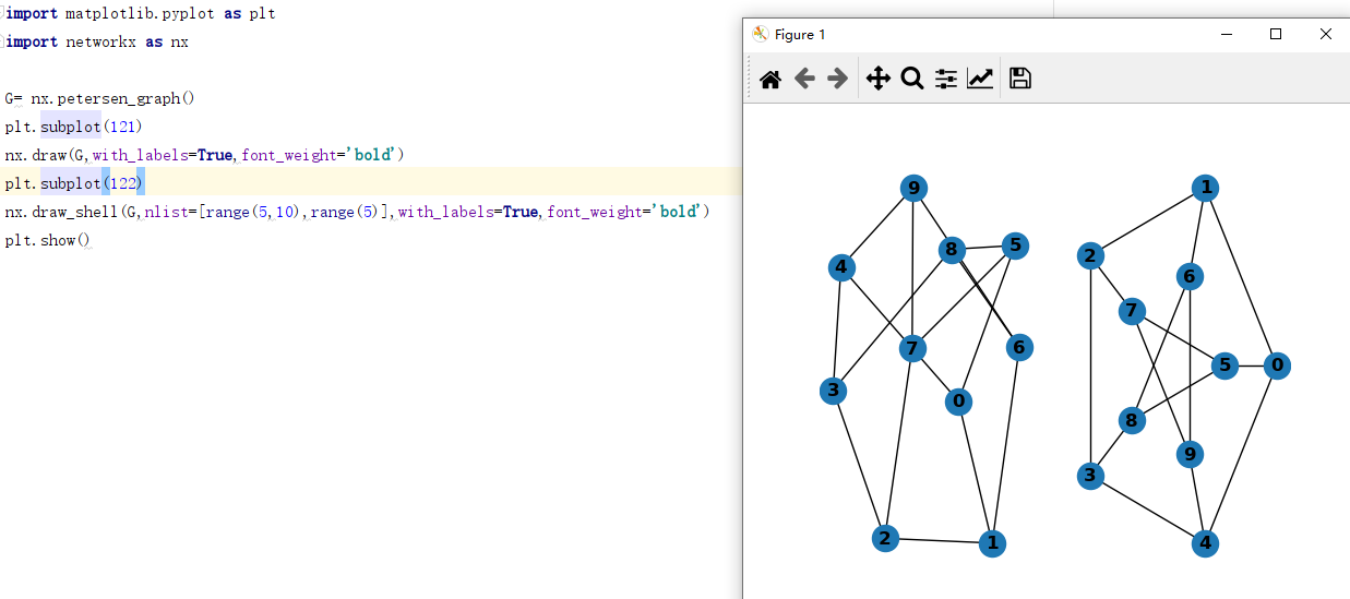
  • 各种经典小图数据。如彼得森图networkx.petersen_graph()会生成一个有固定节点和边的彼得森图
  • 也可以按照给定节点数生成其他经典图，如5个节点的完全图networkx.complete_graph(5),完全二分图nx.complete_bipartite_graph(3, 5)
  • 随机图生成器：er = nx.erdos_renyi_graph(100, 0.15),red = nx.random_lobster(100, 0.9, 0.9)等。
  • 从数据源格式读取：支持各种图存储格式读取。边列表，邻居列表，GML,GraphML,pickle,LEDA等。

• 分析图：可以对图做各种分析，比如连通图分析，最短路径分析等。所有支持的计算算法 特别多。。

• 画图：此包并非用于画图，但是可以用Python matplotlib和Graphviz软件包接口一起画图。

5 使用Python实际分析网络数据

5.1 构建网络

参考教程

载入相关包和数据

import csv
from operator import itemgetter
import networkx as nx
#This part of networkx, for community detection, needs to be imported separately.
from networkx.algorithms import community 
# 载入数据，假设节点名称列表和边列表分别位于两个不同的csv文件 quakers_nodelist.csv 和 quakers_edgelist.csv
with open('quakers_nodelist.csv', 'r') as nodecsv:                      
    nodereader = csv.reader(nodecsv)    
    nodes = [n for n in nodereader][1:]                     

node_names = [n[0] for n in nodes] # Get a list of only the node names                                       

with open('quakers_edgelist.csv', 'r') as edgecsv:
    edgereader = csv.reader(edgecsv)      
    edges = [tuple(e) for e in edgereader][1:]

创建网络图，并加入节点和边,并输出基本信息

G = nx.Graph()
G.add_nodes_from(nodes)
G.add_edges_from(edges)
print(nx.info(G))

得到网络基本信息

Name:
Type: Graph
Number of nodes: 119
Number of edges: 174
Average degree: 2.9244

假若上述的节点信息列表包含了其他列，比如name,historical significance,gender,birth year,death year,SDFB ID属性，你想将这些属性也加入到网络中。networkx允许给节点和边添加属性nx.set_node_attributes()和nx.set_edge_attributes()。你需要将这些属性转化为词典形式，key为节点名，value为属性值，需要对每个属性创建一个词典。

hist_sig_dict = {}
gender_dict = {}
birth_dict = {}
death_dict = {}
id_dict = {}

循环遍历所有节点，给不同属性赋值

# 一个节点有多列，依次为 name,historical significance,gender,birth year,death year,SDFB ID
for node in nodes: # Loop through the list, one row at a time
    hist_sig_dict[node[0]] = node[1] 
    gender_dict[node[0]] = node[2]
    birth_dict[node[0]] = node[3]
    death_dict[node[0]] = node[4]
    id_dict[node[0]] = node[5]

然后通过set_node_attributes将所有属性词典添加到网络图

nx.set_node_attributes(G, hist_sig_dict, 'historical_significance')
nx.set_node_attributes(G, gender_dict, 'gender')
nx.set_node_attributes(G, birth_dict, 'birth_year')
nx.set_node_attributes(G, death_dict, 'death_year')
nx.set_node_attributes(G, id_dict, 'sdfb_id')
# 测试访问节点的birth_year属性
for n in G.nodes(): 
    print(n, G.nodes[n]['birth_year'])

5.2 网络分析

分析之前我们需要知道要分析的网络数据的大体情况，比如有多少节点，多少边。节点太少(小于15个节点，不如直接画出来)或太多(比如150万个节点，分析子集)都不利于分析。当前无向图网络相对于有向图更容易分析。

5.2.1 网络图外观

网络图外观显示了节点之间如何连接的，因为网络图有拓扑结构，可以看出连接关系，数据分布中心化还是去中心化的，稠密的还是稀疏的，圆形 还是线型连接居多，是聚合在一起还是分散的。当前分析的数据集(Quaker)使用Gephi(Force-directed分布(对于小数据集可以创建干净、易于理解的图))可视化效果如下

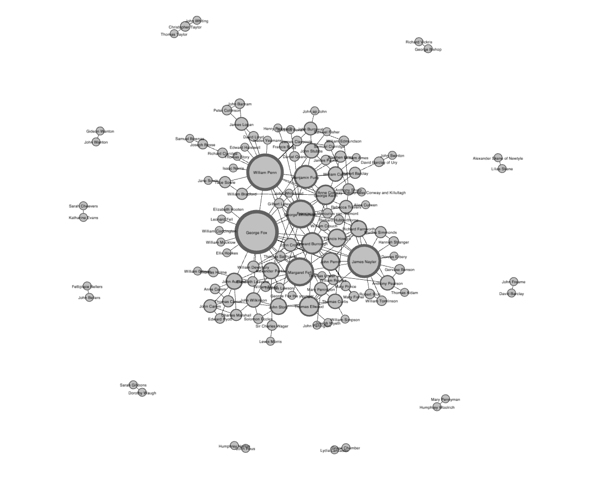
可视化能分析到的东西基本到此为止。更详细的分析需要量化。

• 稠密度(density):一个不错的开始分析指标。所有节点实际边数目除以所有可能连接数。此参数可以让你快速了解网络连接情况。nx.density(G)
• 最短路径分析：相对复杂，并且在大网络可视化时不容易发现。主要适用于找到朋友的朋友，参考六度定律。假若我们要计算节点A到B之间最短路径。nx.shortest_path(G, source="A", target="B")，会输出从A到B节点的中间节点列表。如果某个节点是位于很多最短路径中间，此节点一般是Hub,并且重要性较高。
  • 半径：顺着最短路径分析，可以分析很多其他指标。比如半径(diameter),如果直接对当前网络计算半径会出错，因为网络包含很多子图，子图之间不连通。可以分析网络找到最大连通图，然后计算其半径。components = nx.connected_components(G);largest_component = max(components, key=len)。如果最大连通图的半径为8，表明最长的最短路径为8.
• 三重闭合度(triadic closure):如果两个人都认识同一个人，那么这两个人也可能彼此认识，这会在网络中形成一个三角形。网络中这些闭合三角形的数量可以用于发现网络中聚类簇和社区。nx.transitivity(G)
  • 聚类系数clustering coefficient：衡量网络中三角闭合度的一般称为聚类系数，因为它表示的是聚集的倾向。但是结构化的网络图使用的是transitivity代表的是所有存在的三角数量除以所有可能的三角数量的比例。刻画的是网络内部的连接。
  • 切记，考察如transitivity和稠密度(density)时多考虑似然度(likehoods)而非certainties。transitivity让你能顺着连接性理解网络，

5.2.2 中心度

下一步是分析网络中哪些节点比较重要。分析节点重要程度的方法有很多。包括degree(度),betweenness centrality(中介性),eigenvector centrality(特征向量中心性)。

有较多度数的节点称之为hub，计算节点度数是找到hub的最快方法。这些hub是网络中关键，比如当前数据集中最高度数的节点是此关系网创建人，其他度数少一些的是共同创建人。

# 计算所有节点的度，然后将其作为网络属性词典
degree_dict = dict(G.degree(G.nodes()))
nx.set_node_attributes(G, degree_dict, 'degree')
print(G.nodes['William Penn'])
# 对所有节点按照度从大到小排序
import itemgetter
# itemgetter(1) 代表要对degree_dict.items中第2个列排序
sorted_degree = sorted(degree_dict.items(), key=itemgetter(1), reverse=True)

eigenvector centrality(特征向量中心性)是度数的一种拓展，结合了节点的边以及节点的邻居。它计算的是如果你是一个hub，以及你与都少个hub连接。其取值范围是0到1,值越大越具有中心性。对于理解哪些节点能迅速传递信息十分有帮助。PageRanke算法是特征向量中心性的拓展。

betweenness centrality(介中性)与另外两种度量方法不同，它不关心某个/些节点的边数目。它关心的是所有通过单个节点的最短路径。为计算这些最短路径，首先得计算网络中所有可能的最短路径，所以此度量计算比较耗时，其取值范围也是0到1。使用它很容易找到网络中分离的两个子网。如果两个聚类簇之间仅存在一个节点，这两个聚类簇之间的所有社区都必须经过此节点。与hub相反，此节点称之为broker。尽管介中性不是发现broker的唯一手段，但是是最有效率的。它让你知道，某些节点虽然与它们相连的节点数少，但是它们是网络子网之间桥梁

betweenness_dict = nx.betweenness_centrality(G) # Run betweenness centrality
eigenvector_dict = nx.eigenvector_centrality(G) # Run eigenvector centrality
# 将属性赋予网络
nx.set_node_attributes(G, betweenness_dict, 'betweenness')
nx.set_node_attributes(G, eigenvector_dict, 'eigenvector')
# 根据介中性 排序
sorted_betweenness = sorted(betweenness_dict.items(), key=itemgetter(1), reverse=True)
print("Top 20 nodes by betweenness centrality:")
for b in sorted_betweenness[:20]:
    print(b)

</div