PyTorch Geometric vs. Deep Graph Library

A Comparison Between Graph Neural Networks: DGL vs. PyTorch Geometric

What is deep learning on graphs?

In general, a graph is a system of nodes connected by edges. The nodes typically have some sort of internal state that can be modified by the relationships to other nodes defined by the edges connecting them to other nodes, and these connections and node states can be defined in a wide variety of ways.

Deep learning is the repeated application of non-linear transformations to data (representations or activations internally), which are often matrix multiplications or convolutions. Combining deep learning and graphs gives us the fast-growing field of graph neural networks (GNNs).

Graphs provide a useful framework for any system readily defined by nodes and relationships, including social networks, molecules, and many other types of real and theoretical systems. Working with data defined as graphs imparts meaningful structural data to the system under study, and is accompanied by a rich toolbox of available mathematical and algorithmic tools.

What’s more, because graphs can be described and manipulated with matrix math, they make a fitting complement to deep learning and benefit greatly from the years of development of fast deep learning libraries which use mainly the same mathematical primitives.

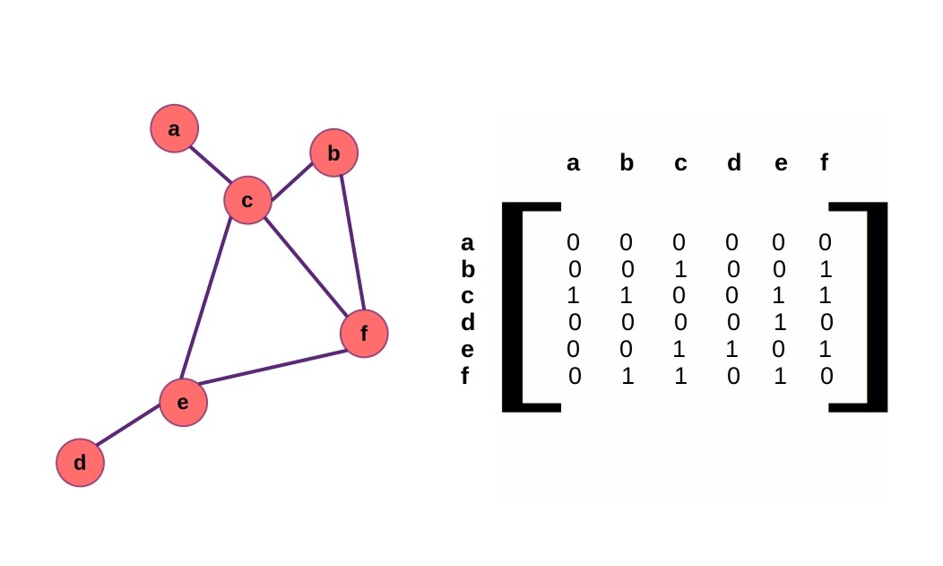
An adjacency matrix represents the edge connections in a graph. Public domain diagram by rivesunder.

Given the rich framework provided by graphs for many types of problems and the substantial successes of deep learning neural networks over the past few decades, it’s no surprise that graph neural networks (GNNs in this article) have garnered increasingly levels of attention and the field has generated its own specialized breakthroughs.

Arguably the most exciting accomplishment of deep learning with graphs so far has been the development of AlphaFold and AlphaFold2 by DeepMind, a project that has made major strides in solving the protein structure prediction problem, a long-standing grand challenge of structural biology.

With myriad important applications in drug discovery, social networks, basic biology, and many other areas, a number of open-source libraries have been developed for working with graph neural networks.

Many of these are mature enough to use in production or research, so how can you go about choosing which library to use when embarking on a new project? Various factors can contribute to the choice of GNN library for a given project.

Not least of all is the compatibility with you and your team’s existing expertise: if you are primarily a PyTorch shop it would make sense to give special consideration to PyTorch Geometric, although you might also be interested in using the Deep Graph Library with PyTorch as the backend (DGL can also use TensorFlow as a backend).

Likewise, if you are more familiar with TensorFlow and Keras, Spektral may make sense. If you want to develop with the up-and-coming JAX ecosystem, then Jraph might be a good fit for your GNN project.

Of course, if your team prefers to work in Julia instead of Python, you would probably want to look at GeometricFlux.jl or GraphNeuralNetworks.jl, both based on the Flux.jl machine learning ecosystem.

Like other tools written in Julia and the Julia programming language itself, GeometricFlux.jl and GraphNeuralNetworks.jl are not as well-known and have smaller communities than the more established Python counterparts, but they do offer a few compelling advantages as well. Among the most desirable advantages of Julia-based tools is execution speed, thanks to Julia’s built-in "just-in-time" compilation.

While existing familiarity with a given language and similar libraries like PyTorch or TensorFlow contribute significantly to the efficiency of development in terms of the engineering time required to complete a given task, the other major contributor to efficiency in a machine learning project (and the more obvious and recognized of the two) is computational speed.

Developer time tends to be a scarce resource and often underestimated constraint in machine learning projects than execution speed of the code itself, but imagine how much longer it would take for the impacts of deep learning to mature if we didn’t have widely available libraries for efficient hardware acceleration on GPUs (and more esoteric and specialized devices).

Yet all the specialized hardware in the world won’t do much good without efficient software implementations to match.

In this article, we will benchmark and compare two of the most noteworthy open-source libraries for computing with graph neural networks. For the purposes of this comparison, we’ll focus on Python libraries PyTorch Geometric and Deep Graph Library (DGL). As the name implies, PyTorch Geometric is based on PyTorch (plus a number of PyTorch extensions for working with sparse matrices), while DGL can use either PyTorch or TensorFlow as a backend.

DGL was used to develop the SE3-Transformer, a translationally and rotationally invariant model that heavily influenced the protein-structure prediction champion model AlphaFold. DGL is also used in the Baker lab’s open-source RosettaFold protein structure prediction inspired by DeepMind’s work.

PyTorch Geometric is a popular library (over 13,000 stars on GitHub) with a conveniently familiar API for anyone with prior PyTorch experience. We’ll introduce the APIs for each and benchmark equivalent GNN architectures on a protein-protein interaction (PPI) dataset from Zitnik and Leskovec’s 2017 publication.

The PPI dataset presents a multiclass node classification task, each node represents one protein by 50 features and is labeled with 121 non-exclusive labels.

If you have been working with deep learning models for a while, you have probably experienced the wax and wane of popular Python libraries. Prior to the widespread adoption of TensorFlow following Google’s release of the open-source library in 2015 (pdf), the deep learning library landscape was a multivariate affair of frameworks like Theano, AutoGrad, Caffe, Lasagne, Keras, Chainer, and others.

Just a few years before that, libraries were mostly roll-your-own. If you wanted GPU support, you probably had to know CUDA. PyTorch was introduced in 2016 and slowly but surely became the preferred library for research, while TensorFlow swallowed Keras and remained favored for production workflows.

By the time TensorFlow released version 2.0, it seemed like deep learning in Python was a two-library game with the differences between them diminishing, with TensorFlow becoming more dynamic like PyTorch and PyTorch getting faster with just-in-time compilation and the development of Torchscript.

Perhaps because of the trend to convergence of the two major libraries, JAX, a successor to the academic project Autograd, found an open niche for capable, functional, and composable deep learning. JAX is rapidly gaining interest from major research labs like DeepMind.

Jraph is DeepMind’s JAX-based answer to graph-based deep learning, though it shares many characteristics of their previous project in TensorFlow, Graph Nets, which as of this writing, hasn’t been updated for just over a year.

In the next section, we’ll look at how to install and setup DGL and PyTorch Geometric, and how to build a graph convolutional network with 6 hidden layers using each library. We’ll also set up a training loop for learning node classification on the PPI dataset for each and discuss some differences in the graph data structure API used by each. Finally, we execute a 10,000 epoch training run on a single NVIDIA GPU and compare the speed of each.

PyTorch Geometric

PyTorch Geometric (PyG) is an intuitive library that feels much like working with standard PyTorch. The datasets and dataloaders have a consistent API, so there's no need to manually adjust model architectures for different tasks.

Install

Note that we installed PyTorch Geometric based on a system setup with pip, PyTorch 1.10, Python 3.6, and CUDA 10.2. If you have different requirements, you can easily determine if your setup commands will look different by putting your system's info into the instructions in the documentation.

virtualenv pyg_env –-python=python3 
source pyg_env/bin/activate 
pip install torch==1.10.0 
pip install torch-scatter torch-sparse torch-cluster \
   torch-spline-conv \
   torch-geometric -f https://data.pyg.org/whl/torch-1.10.0+cu102.html

Model and Code

The architecture we’ll use for benchmarking these libraries is based on the graph convolutional layers described by Kipf and Welling in their 2016 paper (GCNConv in PyTorch Geometric, and GraphConv in DGL).

Graph layers in PyTorch Geometric use an API that behaves much like layers in PyTorch, but take as input the graph edges stored in edge_index in the PyTorch Geometric Batch class. Batches in the library describe an agglomeration of one or more graphs as one big graph that just happens to have a few internal gaps.

For graph convolutions, these batches use matrix-multiplication and a combined adjacency matrix to accomplish weight-sharing, but the Batch object also keeps track of which node belongs to which graph in a variable called batch.

The graph convolutional model we'll be using looks like the following diagram:

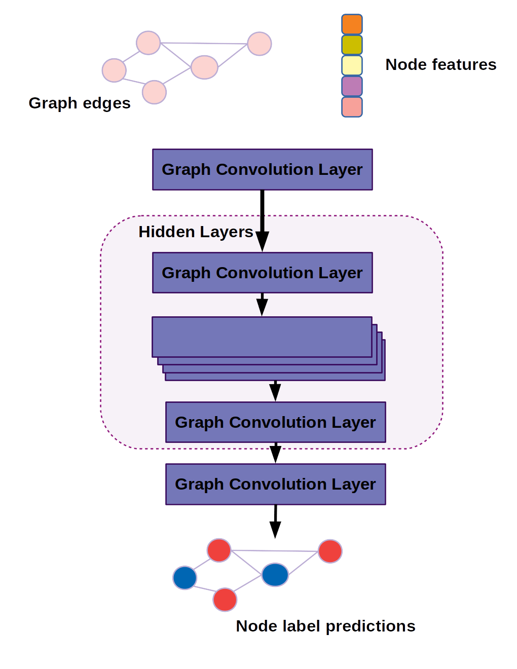
Diagram of the graph convolutional network used to benchmark DGL and PyTorch Geometric.

In code, our model is built by inheriting from PyTorch's torch.nn.Module model class.

import time 
import numpy as np 
import torch 
import torch.nn as nn 
import torch_geometric 
from torch_geometric.nn import GCNConv 
from torch_geometric.datasets import PPI 
from torch_geometric.loader import DataLoader
 
class GCNConvNet(nn.Module):
    def __init__(self, in_channels=3, out_channels=6):
     super(GCNConvNet, self).__init__()
     self.gcn_0 = GCNConv(in_channels, 64)
     self.gcn_h1 = GCNConv(64, 64)
     self.gcn_h2 = GCNConv(64, 64)
     self.gcn_h3 = GCNConv(64, 64)
     self.gcn_h4 = GCNConv(64, 64)
     self.gcn_h5 = GCNConv(64, 64)
     self.gcn_h6 = GCNConv(64, 64)
     self.gcn_out = GCNConv(64, out_channels) 

def forward(self, batch):
     x, edge_index, batch_graph = batch.x, batch.edge_index, batch.batch
     x = torch.relu(self.gcn_0(x, edge_index))
     x = torch.relu(self.gcn_h1(x, edge_index))
     x = torch.relu(self.gcn_h2(x, edge_index))
     x = torch.relu(self.gcn_h3(x, edge_index))
     x = torch.relu(self.gcn_h4(x, edge_index))
     x = torch.relu(self.gcn_h5(x, edge_index))
     x = torch.relu(self.gcn_h6(x, edge_index))
     x = torch.dropout(x, p=0.25, train=self.training)
     x = self.gcn_out(x, edge_index)
     x = torch.sigmoid(x)
     return x

Notice that instead of taking a tensor as input, this model takes a variable called "batch," and sometimes more generically called "data" in common style conventions. The batch contains the extra information defining which nodes belong to which graphs and how those nodes are connected.

Aside from that difference, the model reads much like a standard convolutional network, with GCNConv or similar graph-based layers instead of standard convolutions.

The training loop is also very familiar for PyTorch users, but passes the entire batch to the model instead of a lonely input tensor. But before we can get to the training loop we need to download the protein-protein interaction (PPI) dataset and set up our training and test dataloader.

num_epochs = 10000 
lr = 1e-3 

dataset = PPI(root="./tmp") 
dataset = dataset.shuffle()
 
test_dataset = dataset[:2] 
train_dataset = dataset[2:] 

test_loader = DataLoader(test_dataset, batch_size=1) 
train_loader = DataLoader(train_dataset, batch_size=8, shuffle=True) 

for batch in train_loader:
     Break 

in_channels = batch.x.shape[1] 
out_channels = dataset.num_classes 

model = GCNConvNet(in_channels = in_channels,\
         out_channels = out_channels) 
loss_fn = torch.nn.BCELoss() 
optimizer = torch.optim.Adam(model.parameters(), lr=lr) 
my_device = "cuda" if torch.cuda.is_available() else "cpu" 
model = model.to(my_device)

Now we are ready to define the training loop. We also keep track of the wall time and loss at each epoch.

losses = [] 
time_elapsed = [] 
epochs = [] 
t0 = time.time() 

for epoch in range(num_epochs): 

     total_loss = 0.0
     batch_count = 0
     for batch in train_loader: 
        optimizer.zero_grad() 
        pred = model(batch.to(my_device)) 
        loss = loss_fn(pred, batch.y.to(my_device)) 
        loss.backward() 
        optimizer.step() 
        total_loss += loss.detach() 
        batch_count += 1 

    mean_loss = total_loss / batch_count 
    losses.append(mean_loss) 
    epochs.append(epoch) 
    time_elapsed.append(time.time()-t0) 
    if epoch % 100 == 0: 
        print(f"loss at epoch {epoch} = {mean_loss}")

That's it; the code is ready for benchmarking PyTorch Geometric on the PPI dataset. With that in place, building an equivalent model in Deep Graph Library will be much easier, because there are only a few differences in the code which we'll attend to in the next section.

The Deep Graph Library (DGL)

Deep Graph Library is a flexible library that can utilize PyTorch or TensorFlow as a backend. We'll use PyTorch for this demonstration, but if you normally work with TensorFlow and want to use it for deep learning on graphs you can do so by exporting 'tensorflow' to an environmental variable named DGLBACKEND.

At a minimum, you'll likely also want to adapt the code to subclass from tf.keras.Model instead of torch.nn.Module, and to use the fit API from keras. API in keras, for example.

Install

Once again, we're installing on a system with CUDA 10.2, but if you have upgraded to CUDA 11 or are still stuck on CUDA 10.1 you can get the proper pip install command from the DGL website.

virtualenv dgl_env –python=python3 
source dgl_env/bin/activate 
pip install torch=1.10.0 

pip install dgl-cu102 -f https://data.dgl.ai/wheels/repo.html

Model and Code

In DGL, the Kipf and Welling graph convolution layer is called 'GraphConv' instead of 'GCNConv' as used in PyTorch Geometric. Aside from that, the model will look mostly the same.

import time 
import numpy as np 
import torch 
import torch.nn as nn 

import dgl 
from dgl.nn import GraphConv 
from dgl.data import PPIDataset 
from dgl.dataloading.pytorch import GraphDataLoader 
from dgl.data.utils import split_dataset 

class GraphConvNet(nn.Module): 

    def __init__(self, in_channels=3, out_channels=6): 
        super(GraphConvNet, self).__init__() 

        self.gcn_0 = GraphConv(in_channels, 64,\ 
        allow_zero_in_degree=True) 

        self.gcn_h1 = GraphConv(64, 64, allow_zero_in_degree=True) 
        self.gcn_h2 = GraphConv(64, 64, allow_zero_in_degree=True) 
        self.gcn_h3 = GraphConv(64, 64, allow_zero_in_degree=True) 
        self.gcn_h4 = GraphConv(64, 64, allow_zero_in_degree=True) 
        self.gcn_h5 = GraphConv(64, 64, allow_zero_in_degree=True) 
        self.gcn_h6 = GraphConv(64, 64, allow_zero_in_degree=True) 

        self.gcn_out = GraphConv(64, out_channels, \ 
        allow    _zero_in_degree=True)
 
    def forward(self, g, features): 

        x = torch.relu(self.gcn_0(g, features)) 

        x = torch.relu(self.gcn_h1(g, x)) 
        x = torch.relu(self.gcn_h2(g, x)) 
        x = torch.relu(self.gcn_h3(g, x)) 
        x = torch.relu(self.gcn_h4(g, x)) 
        x = torch.relu(self.gcn_h5(g, x)) 
        x = torch.relu(self.gcn_h6(g, x)) 

        x = torch.dropout(x, p=0.25, train=self.training) 
        x = self.gcn_out(g, x) 

        x = torch.sigmoid(x) 

        return x

Note that instead of passing batch as the input, we pass g (the DGL graph object) and the node features.

In setting up the training loop, the outline is mostly the same as well, but pay careful attention to what gets passed to the model.

In this case the node features are found in 'batch.ndata["feat"]' but we've found that the specific key used for the node features varies between datasets. 'feat' is probably the most common, but you'll also find 'node_attr' and others and the inconsistent API can be a little confusing.

This was a significant pain point while we experimented with different built-in datasets for this demo, and re-writing bits of the code to fit different datasets can really slow down development. We certainly came to appreciate the consistency of the 'Batch' object used in PyTorch Geometric.

In practice, consistent internal styling would make this a non-issue in a real-world application, since you wouldn't be using the built in datasets anyway.

if __name__ == "__main__": 
    num_epochs = 10000 
    lr = 1e-3 
    my_seed = 42 

    dataset = PPIDataset() 

    # randomly create dataset split 
    test_dataset, train_dataset = split_dataset(dataset, [0.1, 0.9],\ 
    shuffle=True) 
    train_loader = GraphDataLoader(train_dataset, batch_size=8) 
    test_loader = GraphDataLoader(test_dataset, batch_size=1) 

    for batch in train_loader: 
    break 

    in_channels = batch.ndata["feat"].shape[1] 
    out_channels = dataset.num_labels 
    model = GraphConvNet(in_channels, out_channels) 

    loss_fn = torch.nn.BCELoss() 
    optimizer = torch.optim.Adam(model.parameters(), lr=lr) 
    my_device = "cuda" if torch.cuda.is_available() else "cpu" 

    model = model.to(my_device) 

    losses = [] 
    time_elapsed = [] 
    epochs = [] 
    t0 = time.time() 

    for epoch in range(num_epochs): 

        total_loss = 0.0 
        batch_count = 0 

        for batch in train_loader: 
            optimizer.zero_grad() 
            batch = batch.to(my_device) 
            pred = model(batch, batch.ndata["feat"].to(my_device)) 
            loss = loss_fn(pred, batch.ndata["label"].to(my_device)) 
            loss.backward() 
            optimizer.step() 

            total_loss += loss.detach() 
            batch_count += 1 

        mean_loss = total_loss / batch_count 
        losses.append(mean_loss) 
        epochs.append(epoch) 
        time_elapsed.append(time.time() - t0) 

        if epoch % 100 == 0: 
            print(f"loss at epoch {epoch} = {mean_loss}") 

    # get test accuracy score 
    num_correct = 0. 
    num_total = 0. 
    model.eval() 

    for batch in test_loader: 

        batch = batch.to(my_device) 
        pred = model(batch, batch.ndata["feat"]) 
        num_correct += (pred.round() == \ 
            batch.ndata["label"].to(my_device)).sum() 
        num_total += pred.shape[0] * pred.shape[1] 

        np.save("dgl.npy", \ 
            {"epochs": epochs, \ 
            "losses": losses, \ 
            "time_elapsed": time_elapsed}) 

    print(f"test accuracy = {num_correct / num_total}")

Results

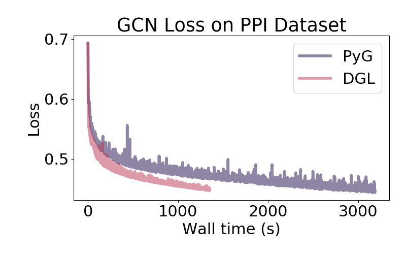
Training curves for DGL and PyTorch Geometric graph convolutional networks on the PPI dataset.

We completed training runs with PyTorch Geometric and DGL for 10,000 epochs each on the PPI dataset, running on a single NVIDIA GTX 1060 GPU.

PyG took 2,984.34 seconds to complete training, while DGL took less than half as long at 1,148.05 seconds.

Both runs ended with similar performance, with test accuracy of 73.35% for PyG and 77.38% for DGL, which is within the kind of difference we would expect to occur by chance by random initialization for different runs.

After 10,000 epochs loss was still decreasing, so you could expect this model architecture to eventually converge on a slightly higher accuracy (though we weren't tracking a validation loss for this experiment).

Deciding Which GNN Library Is Right for You

We were surprised by how big the difference in training times was between libraries. Given that both DGL and PyG are built on PyTorch or use PyTorch as the computational back end, it was expected they would both finish within about 10% or 20% of each other.

We did find setting up the training loop with PyTorch Geometric to be much more enjoyable than with DGL, as the batch API is more intuitive and consistent than the equivalent in DGL. We tried out several different datasets before settling on the PPI dataset, and it seemed like each one used a different key to retrieve node features using DGL.

That being said, the minor annoyances experienced with DGL probably have as much to do with our familiarity with the library as anything, as we've used PyG longer than DGL.

Although it would be worth examining a few different architectures and layer types for performance (tailored to your specific use case), it's hard to argue with a 2X performance boost just from choosing the right library.

Although developer time is generally a scarcer resource than computational time, DGL was nearly 2.6 times faster in this setup, and that's an advantage that is probably worth training up and switching libraries. It's likely that whatever small annoyances experienced with the DGL ecosystem would vanish with better familiarity.

Although DGL is currently a little less popular than PyTorch Geometric as measured by GitHub stars and forks (13,700/2,400 vs 8,800/2,000), there is plenty of community support to ensure the library is easy enough to learn and troubleshoot, and the documentation is also pretty good.

Whatever you decide, it's clear that learning from the structural information encoded in graphs has a lot to offer learning in any context where data is generated in a network format, and improvements in hardware and software support for fast computation with sparse matrices continues to make the investment in developing with GNN libraries worthwhile.