

What Is the Second Difference Matrix?
source link: https://nhigham.com/2022/01/31/what-is-the-second-difference-matrix/
Go to the source link to view the article. You can view the picture content, updated content and better typesetting reading experience. If the link is broken, please click the button below to view the snapshot at that time.

What Is the Second Difference Matrix?
The second difference matrix is the tridiagonal matrix 


![\notag T_n = \left[ \begin{array}{@{}*{4}{r@{\mskip10mu}}r} 2 & -1 & & & \\ -1 & 2 & -1 & & \\[-5pt] & -1 & 2 & \ddots & \\ & & \ddots & \ddots & -1 \\ & & & -1 & 2 \end{array}\right] \in\mathbb{R}^{n\times n}.](https://s0.wp.com/latex.php?latex=%5Cnotag++++T_n+%3D+%5Cleft%5B++++%5Cbegin%7Barray%7D%7B%40%7B%7D%2A%7B4%7D%7Br%40%7B%5Cmskip10mu%7D%7Dr%7D+++++++++++++++++2++%26+-1+%26++++++++%26++++++++%26++++%5C%5C+++++++++++++++++-1+%26+2++%26+-1+++++%26++++++++%26++++%5C%5C%5B-5pt%5D++++++++++++++++++++%26+-1+%26+2++++++%26+%5Cddots+%26++++%5C%5C++++++++++++++++++++%26++++%26+%5Cddots+%26+%5Cddots+%26+-1+%5C%5C++++++++++++++++++++%26++++%26++++++++%26+-1+++++%26+2++++%5Cend%7Barray%7D%5Cright%5D+%5Cin%5Cmathbb%7BR%7D%5E%7Bn%5Ctimes+n%7D.+&bg=ffffff&fg=222222&s=0&c=20201002)
It arises when a second derivative is approximated by the central second difference 

gallery('tridiag',n), which is returned as a aparse matrix.
This is Gil Strang’s favorite matrix. The photo, from his home page, shows a birthday cake representation of the matrix.

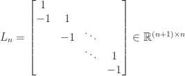
The second difference matrix is symmetric positive definite. The easiest way to see this is to define the full rank rectangular matrix
and note that 

Cholesky Factorization
In an LU factorization 


Determinant, Inverse, Condition Number
Since the determinant is the product of the pivots, 
The inverse of 

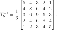
The 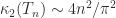
Eigenvalues and Eigenvectors
The eigenvalues of

where 

The matrix 
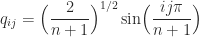
is therefore an eigenvector matrix for 
Variations
Various modifications of the second difference matrix arise and similar results can be derived. For example, consider the matrix obtained by changing the 

![\notag \widetilde{T}_n = \left[ \begin{array}{@{}*{4}{r@{\mskip10mu}}r} 2 & -1 & & & \\ -1 & 2 & -1 & & \\[-5pt] & -1 & 2 & \ddots & \\ & & \ddots & \ddots & -1 \\ & & & -1 & 1 \end{array}\right] \in\mathbb{R}^{n\times n}.](https://s0.wp.com/latex.php?latex=%5Cnotag++++%5Cwidetilde%7BT%7D_n+%3D+%5Cleft%5B++++%5Cbegin%7Barray%7D%7B%40%7B%7D%2A%7B4%7D%7Br%40%7B%5Cmskip10mu%7D%7Dr%7D+++++++++++++++++2++%26+-1+%26++++++++%26++++++++%26++++%5C%5C+++++++++++++++++-1+%26+2++%26+-1+++++%26++++++++%26++++%5C%5C%5B-5pt%5D++++++++++++++++++++%26+-1+%26+2++++++%26+%5Cddots+%26++++%5C%5C++++++++++++++++++++%26++++%26+%5Cddots+%26+%5Cddots+%26+-1+%5C%5C++++++++++++++++++++%26++++%26++++++++%26+-1+++++%26+1++++%5Cend%7Barray%7D%5Cright%5D+%5Cin%5Cmathbb%7BR%7D%5E%7Bn%5Ctimes+n%7D.+&bg=ffffff&fg=222222&s=0&c=20201002)
It can be shown that 


If we perturb the 


![\notag \widehat{T}_n = \left[ \begin{array}{@{}*{4}{r@{\mskip10mu}}r} 3 & -1 & & & \\ -1 & 2 & -1 & & \\[-5pt] & -1 & 2 & \ddots & \\ & & \ddots & \ddots & -1 \\ & & & -1 & 1 \end{array}\right] \in\mathbb{R}^{n\times n}.](https://s0.wp.com/latex.php?latex=%5Cnotag++++%5Cwidehat%7BT%7D_n+%3D+%5Cleft%5B++++%5Cbegin%7Barray%7D%7B%40%7B%7D%2A%7B4%7D%7Br%40%7B%5Cmskip10mu%7D%7Dr%7D+++++++++++++++++3++%26+-1+%26++++++++%26++++++++%26++++%5C%5C+++++++++++++++++-1+%26+2++%26+-1+++++%26++++++++%26++++%5C%5C%5B-5pt%5D++++++++++++++++++++%26+-1+%26+2++++++%26+%5Cddots+%26++++%5C%5C++++++++++++++++++++%26++++%26+%5Cddots+%26+%5Cddots+%26+-1+%5C%5C++++++++++++++++++++%26++++%26++++++++%26+-1+++++%26+1++++%5Cend%7Barray%7D%5Cright%5D+%5Cin%5Cmathbb%7BR%7D%5E%7Bn%5Ctimes+n%7D.+&bg=ffffff&fg=222222&s=0&c=20201002)
The inverse is 


Notes
The factorization 
For a derivation of the eigenvalues and eigenvectors see Todd (1977, p. 155 ff.). For the eigenvalues of
References
This is a minimal set of references, which contain further useful references within.
- J. Fortiana and C. N. Cuadras, A Family of Matrices, the Discretized Brownian Bridge, and Distance-Based Regression, Linear Algebra Appl. 264, 173–188, 1997.
- Morris Newman and John Todd, The Evaluation of Matrix Inversion Programs, J. Soc. Indust. Appl. Math. 6(4), 466–476, 1958.
- Gilbert Strang, Essays in Linear Algebra, Wellesley-Cambridge Press, Wellesley, MA, USA, 2012. Chapter A.3: “My Favorite Matrix”.
- John Todd, Basic Numerical Mathematics, Vol.
Recommend
About Joyk
Aggregate valuable and interesting links.
Joyk means Joy of geeK