

python机器学习_近邻算法_分类Ionosphere电离层数据
source link: https://blog.csdn.net/weixin_48964486/article/details/122896585
Go to the source link to view the article. You can view the picture content, updated content and better typesetting reading experience. If the link is broken, please click the button below to view the snapshot at that time.

本文使用python机器学习库Scikit-learn中的工具,以某网站电离层数据为案例,使用近邻算法进行分类预测。并在训练后使用K折交叉检验进行检验,最后输出预测结果及准确率。过程产生一系列直观的可视化图像。希望文章能够对大家有所帮助。祝大家学习顺利!
1.数据获取
1.点击链接获取数据
数据获取链接
http://archive.ics.uci.edu/ml/datasets/Ionosphere
2.点击Data Floder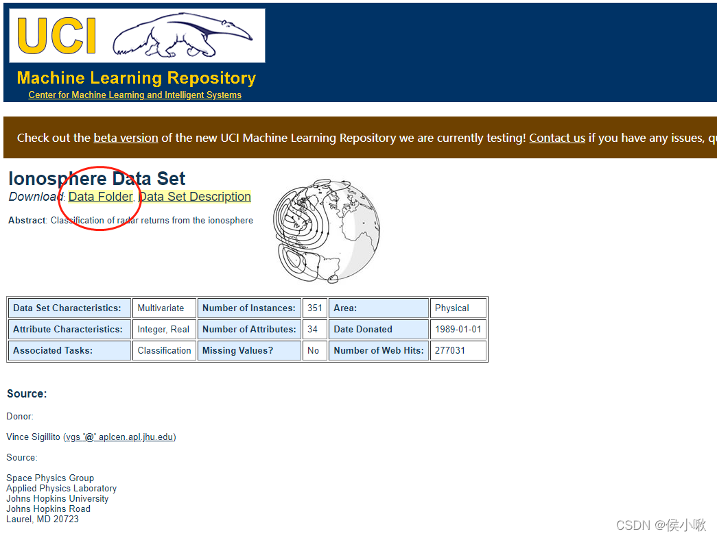
3.选择ionosphere.data和ionosphere.name这两个文件并下载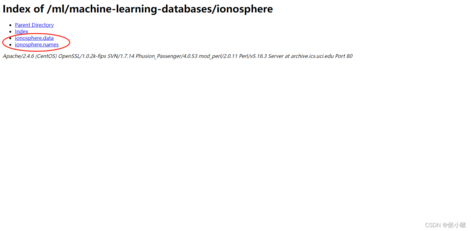
4.下载后放在指定目录下,可以直接通过pycharm查看数据的基本信息
ionosphere.data是我们需要用到的数据,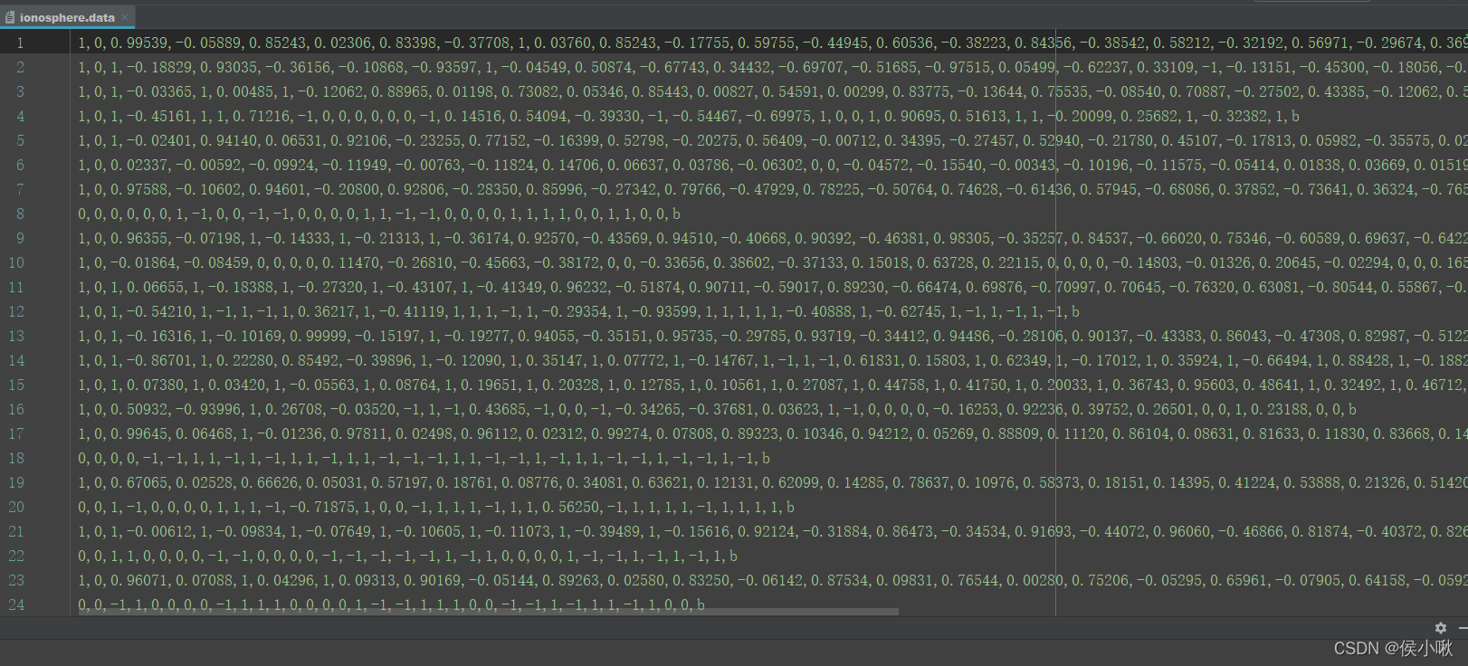
ionosphere.name是对该数据的介绍。
从ionosphere.name中可以看到,ionosphere.data共有351个样本,34个特征,且第35个表示类别,有g和b两个取值,分别表示“good”和“bad”。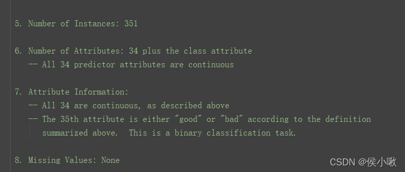
2.数据集分割与初步训练表现
import os
import csv
import numpy as np
from sklearn.model_selection import train_test_split
from sklearn.neighbors import KNeighborsClassifier
from sklearn.model_selection import cross_val_score
from matplotlib import pyplot as plt
from collections import defaultdict


data_filename = "ionosphere.data"


X = np.zeros((351, 34), dtype='float')
y = np.zeros((351,), dtype='bool')


with open(data_filename, 'r') as input_file:
    reader = csv.reader(input_file)
    # print(reader)  # csv.reader类型
    for i, row in enumerate(reader):
        data = [float(datum) for datum in row[:-1]]
        # Set the appropriate row in our dataset
        X[i] = data
        # 将“g”记为1,将“b”记为0。
        y[i] = row[-1] == 'g'


# 划分训练集、测试集
X_train, X_test, y_train, y_test = train_test_split(X, y, random_state=14)

# 即创建估计器(K近邻分类器实例) 默认选择5个近邻作为分类依据
estimator = KNeighborsClassifier()

# 进行训练,
estimator.fit(X_train, y_train)

# 评估在测试集上的表现
y_predicted = estimator.predict(X_test)

# 计算准确率
accuracy = np.mean(y_test == y_predicted) * 100
print("The accuracy is {0:.1f}%".format(accuracy))

# 进行交叉检验,计算平均准确率
scores = cross_val_score(estimator, X, y, scoring='accuracy')
average_accuracy = np.mean(scores) * 100
print("The average accuracy is {0:.1f}%".format(average_accuracy))

如图,该分类算法准确率可达86.4%,交叉检验后的平均准确率可达82.6%。属于是比较优秀的算法。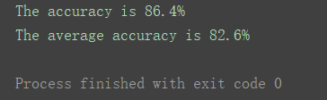
3.测试不同近邻值
测试不同的 近邻数 n_neighbors的值(上边默认为5)下的分类准确率,
选择近邻值从1到20的二十个数字,
并绘图展示
avg_scores = []
all_scores = []
parameter_values = list(range(1, 21))  # Including 20
for n_neighbors in parameter_values:
    estimator = KNeighborsClassifier(n_neighbors=n_neighbors)
    scores = cross_val_score(estimator, X, y, scoring='accuracy')
    avg_scores.append(np.mean(scores))
    all_scores.append(scores)

# 绘制n_neighbors的不同取值与分类正确率之间的关系
plt.figure(figsize=(32, 20))
plt.plot(parameter_values, avg_scores, '-o', linewidth=5, markersize=24)
plt.show()
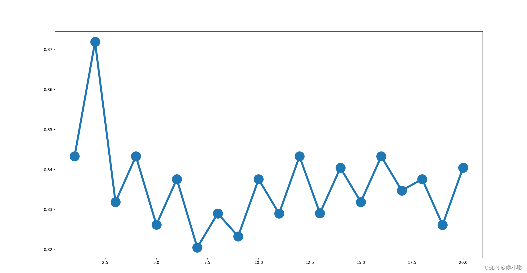
可以看出,准确率整体趋势随着近邻数的增加而减小。近邻值为2时准确率最高。
4.交叉检验
把交叉检验每次验证的准确率也绘制出来
(20个近邻值每个对应5个训练集,对应5次检验)
for parameter, scores in zip(parameter_values, all_scores):
    n_scores = len(scores)
    plt.plot([parameter] * n_scores, scores, '-o')
plt.show()
各次检验准确率图示如下: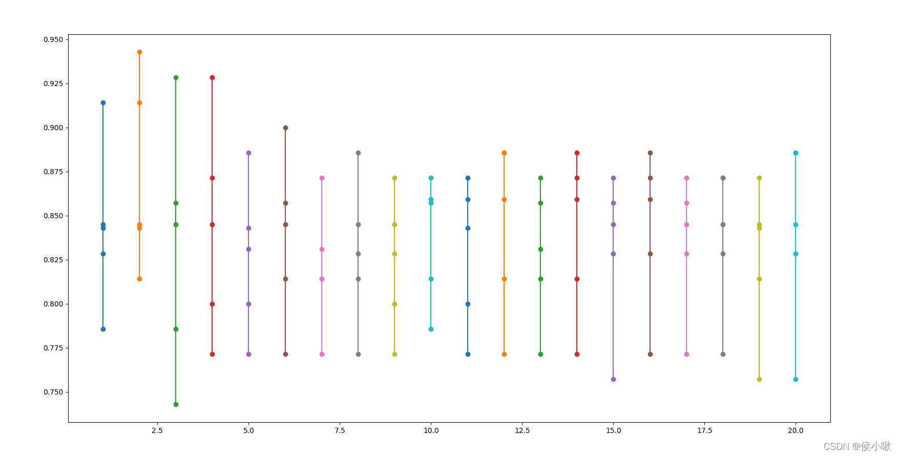
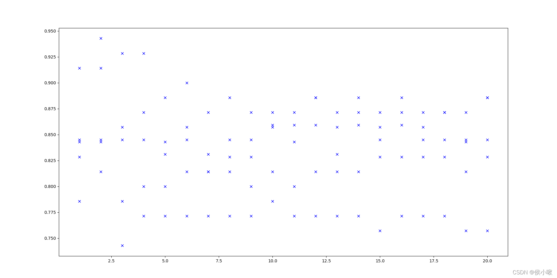
绘制出散点图
plt.plot(parameter_values, all_scores, 'bx')
plt.show()
5. 十折交叉检验
all_scores = defaultdict(list)
parameter_values = list(range(1, 21))  # Including 20

for n_neighbors in parameter_values:
    estimator = KNeighborsClassifier(n_neighbors=n_neighbors)
    scores = cross_val_score(estimator, X, y, scoring='accuracy', cv=10)
    all_scores[n_neighbors].append(scores)

for parameter in parameter_values:
    scores = all_scores[parameter]
    n_scores = len(scores)
    plt.plot([parameter] * n_scores, scores, '-o')

plt.plot(parameter_values, avg_scores, '-o')
plt.show()
检验结果如下图所示: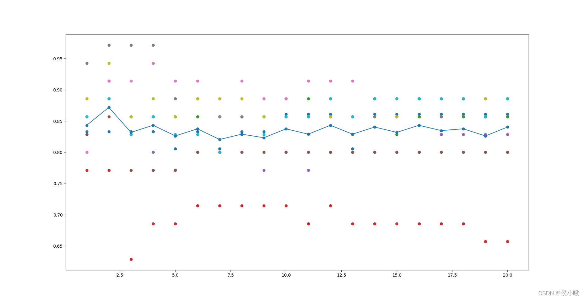
因为每个近邻值下,10次检验中的准确率可能会有重复值,所以在图像中每个近邻值上的准确率个数会有差异。
6.输出预测结果
这里用测试集作为待测数据,使用上述算法进行预测,并输出预测结果,
且令n_neighbors=2
Estimator = KNeighborsClassifier(n_neighbors=2)
Estimator.fit(X_train, y_train)
Y_predicted = Estimator.predict(X_test)
accuracy = np.mean(y_test == Y_predicted) * 100
pre_result = np.zeros_like(Y_predicted, dtype=str)
pre_result[Y_predicted == 1] = 'g'
pre_result[Y_predicted == 0] = 'b'
print(pre_result)
print("The accuracy is {0:.1f}%".format(accuracy))
程序运行结果如下:
如图,预测准确率达92.0%。
Recommend
-
43
-
71
用Scikit-Learn构建K-近邻算法,分类MNIST数据集
-
38
-
26
-
14
开言 从本篇起,将开始我们的机器学习算法系列文章。 机器学习算法的作用不言而喻,是数据挖掘的核心部分也是比较难的一部分。 但是别担心,跟着文章一步步来。
-
24
原创 · 作者 | Giant 学校 | 浙江大学 研究方向 | 对话系统、text2sql 知乎专栏 | 大熊猫游乐园 1、什么...
-
34
↑↑↑关注后" 星标 "Datawhale 每日干货 &
-
29
摘要 :K近邻(k-NearestNeighbor,K-NN)算法是一个有监督的机器学习算法,也被称为K-NN算法,由Cover和Hart于1968年提出,可以用于解决分类问题和回归问题。 为什么要学习k-近邻算法 k...
-
4
K近邻算法的Python实现 作为『十大机器学习算法』之一的K-近邻(K-Nearest Neighbors)算法是思想简单、易于理解的一种分类和回归算法。今天,我们来一起学习KNN算法的基本原理,并用Python实现该算法,最后,通过一个案例阐述其应用价值。 ...
-
4
电离层扰动持续加剧,千寻位置提出“破题”新思路2022/06/02 17:00|
About Joyk
Aggregate valuable and interesting links.
Joyk means Joy of geeK