在处理单个高维数据时,通过可以通过LDA,PCA,等等方法进行降维处理,但是如果某两个数据来自同一个样本,但是数据类型不同,差距巨大时,怎么办呢?这个时候就是典型相关性分析(Canonical Correlation Analysis,CCA)的应用场景.CCA允许我们同时从两套数据分析.典型的应用场景就包括生物学上的联合分析,同一组样本,同时检测转录组和蛋白组,转录组和代谢组以及微生物代谢组等等,更详细的内容可参考维基百科.

CCA与PCA的联系与差别

CCA有点类似PCA(主成分分析,principal component analysis),它们都由同一个课题组提出,在降维方面(canonical variables)可以认为是多套数据的PCA.

不同之处是PCA旨在找出一套数据中能够表示最多方差的线性组合,而CCA旨在找出两套数据中能够最大程度表示其相关性的线性组合.

python实现CCA分析

那么在python中如何实现CCA分析呢? 在sklearn包中的cross_decomposition提供了CCA分析方法,直接调用即可,这里以企鹅数据为例

import pandas as pd
import matplotlib.pyplot as plt
import seaborn as sns
import numpy as np
filename = "penguins.csv"
df = pd.read_csv(filename)
df =df.dropna()
df.head()

species	island	bill_length_mm	bill_depth_mm	flipper_length_mm	body_mass_g	sex
0	Adelie	Torgersen	39.1	18.7	181.0	3750.0	MALE
1	Adelie	Torgersen	39.5	17.4	186.0	3800.0	FEMALE
2	Adelie	Torgersen	40.3	18.0	195.0	3250.0	FEMALE
4	Adelie	Torgersen	36.7	19.3	193.0	3450.0	FEMALE
5	Adelie	Torgersen	39.3	20.6	190.0	3650.0	MALE

我们选取其中两种特征作为研究对象bill_length_mm和bill_depth_mm作为一组,而flipper_length_mm与body_mass_g作为另一组,

from sklearn.preprocessing import StandardScaler
df1 = df[["bill_length_mm","bill_depth_mm"]]
df1_std = pd.DataFrame(StandardScaler().fit(df1).transform(df1), columns = df1.columns)
df1_std.head()
df2 = df[["flipper_length_mm","body_mass_g"]]
df2_std = pd.DataFrame(StandardScaler().fit(df2).transform(df2), columns = df2.columns)
df2_std.head()

# df 1
	bill_length_mm	bill_depth_mm
0	-0.896042	0.780732
1	-0.822788	0.119584
2	-0.676280	0.424729
3	-1.335566	1.085877
4	-0.859415	1.747026
# df2
	flipper_length_mm	body_mass_g
0	-1.426752	-0.568475
1	-1.069474	-0.506286
2	-0.426373	-1.190361
3	-0.569284	-0.941606
4	-0.783651	-0.692852

开始正式的CCA分析

from sklearn.cross_decomposition import CCA
ca = CCA()
xc,yc = ca.fit(df1, df2).transform(df1, df2)

其得到的结果与输入长度一致

np.shape(xc)
# (333,2)
np.shape(yc)
# (333,2)

而且是高度相关的,这里直接计算其相关性

np.corrcoef(xc[:, 0], yc[:, 0])
np.corrcoef(xc[:, 1], yc[:, 1])

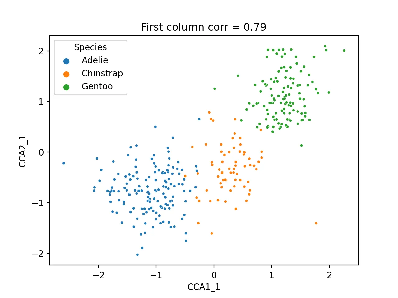
相关性结果为

array([[1.        , 0.78763151],
       [0.78763151, 1.        ]])
array([[1.        , 0.08638695],
       [0.08638695, 1.        ]])

第一对结果很好,相关性0.79,而第二对结果堪忧,我们将CCA分析得到的结果与物种和性别组合成新的dataframe

cca_res = pd.DataFrame({"CCA1_1":xc[:, 0],
                       "CCA2_1":yc[:, 0],
                       "CCA1_2":xc[:, 1],
                       "CCA2_2":yc[:, 1],
                       "Species":df.species,
                      "sex":df.sex})
cca_res.head()

	CCA1_1	CCA2_1	CCA1_2	CCA2_2	Species	sex
0	-1.186252	-1.408795	-0.010367	0.682866	Adelie	MALE
1	-0.709573	-1.053857	-0.456036	0.429879	Adelie	FEMALE
2	-0.790732	-0.393550	-0.130809	-0.839620	Adelie	FEMALE
4	-1.718663	-0.542888	-0.073623	-0.458571	Adelie	FEMALE
5	-1.772295	-0.763548	0.736248	-0.014204	Adelie	MALE

通过其第一列数据进行散点图分析

sns.scatterplot(data=cca_res,x="CCA1_1",y="CCA2_1",hue="Species",s=10)
plt.title(f'First column corr = {np.corrcoef(cca_res.CCA1_1,cca_res.CCA2_1)[0, 1]:.2f}')
plt.savefig("cca_first.png",dpi=200)
plt.close()

其图为: 鉴于第二列数据相关性低,这里通过与原始矩阵进行相关性热图比较,找到其可能的体现的数据

cca_df = pd.DataFrame({"cca1_1":cca_res.CCA1_1,
                        "cca1_2":cca_res.CCA1_2,
                        "cca2_1":cca_res.CCA2_1,
                        "cca2_2":cca_res.CCA2_2,
                        "Species":df.species.astype('category').cat.codes,
                        "Island":df.island.astype('category').cat.codes,
                         "sex":df.sex.astype('category').cat.codes})
dfcor = cca_df.corr()
mask = np.triu(np.ones_like(dfcor))
sns.heatmap(dfcor,cmap="bwr",annot=True)
plt.savefig("cca_corr.png",dpi=200)
plt.close()

绘制的图为:

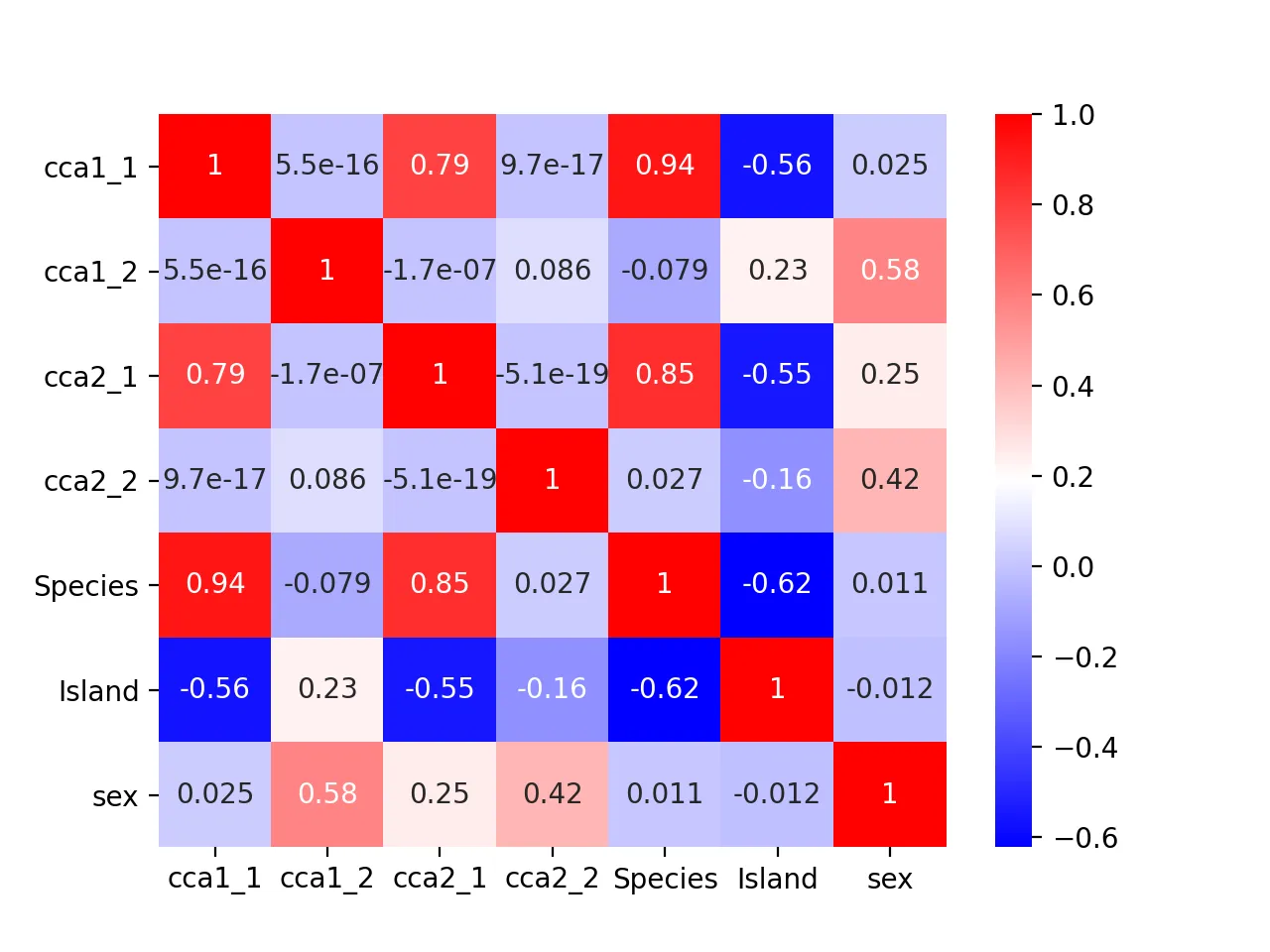
可以看到sex性别与cca2_2相关性最大,为0.42,推测其隐藏信息是性别

sns.scatterplot(data=cca_res,x="CCA1_2",y="CCA2_2",hue="sex",s=10)
plt.title(f'Second column corr = {np.corrcoef(cca_res.CCA1_2,cca_res.CCA2_2)[0, 1]:.2f}')
plt.savefig("cca_sex.png",dpi=200)
plt.close()

图为: 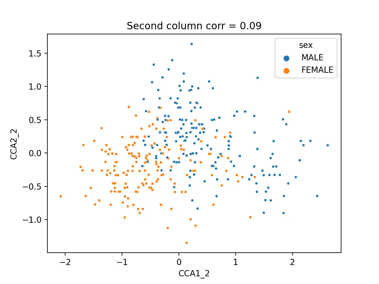不同样本可以明显区分开来,

CCA在高维数据中可以很好的进行多组类型数据的处理,在企鹅数据中表现很好,在生物学上多组学数据的联合分析也是基础的处理方法,后续继续介绍其他的多组学处理方法.