

Blog | Cost Function In MATLAB | MATLAB Helper
source link: https://matlabhelper.com/blog/matlab/cost-function-in-matlab/
Go to the source link to view the article. You can view the picture content, updated content and better typesetting reading experience. If the link is broken, please click the button below to view the snapshot at that time.
Need Urgent Help?
Our experts assist in all MATLAB & Simulink fields with communication options from live sessions to offline work.
testimonials
Philippa E. / PhD Fellow
I STRONGLY recommend MATLAB Helper to EVERYONE interested in doing a successful project & research work! MATLAB Helper has completely surpassed my expectations. Just book their service and forget all your worries.
Yogesh Mangal / Graduate Trainee
MATLAB Helper provide training and internship in MATLAB. It covers many topics of MATLAB. I have received my training from MATLAB Helper with the best experience. It also provide many webinar which is helpful to learning in MATLAB.
Are you working on supervised learning and searching for a method to reduce the error? And do you want to find better values for parameters? Then this blog is for you.
You can reduce errors and can give better values for parameters using cost function and gradient descent. So, without wasting precious time, Let’s discuss these concepts and solutions for these problems.
Introduction:
Before discussing the actual topic, Let’s understand “Hypothesis(h)”. Hypothesis is a function which predict values(h) with given input values(x). For example, An ML (Machine learning) algorithm has to be built to predict the cost price of selling a house, given the size of the site and training data. (This example is considered throughout this blog to understand the concept).

Training data with size and price of the rent house
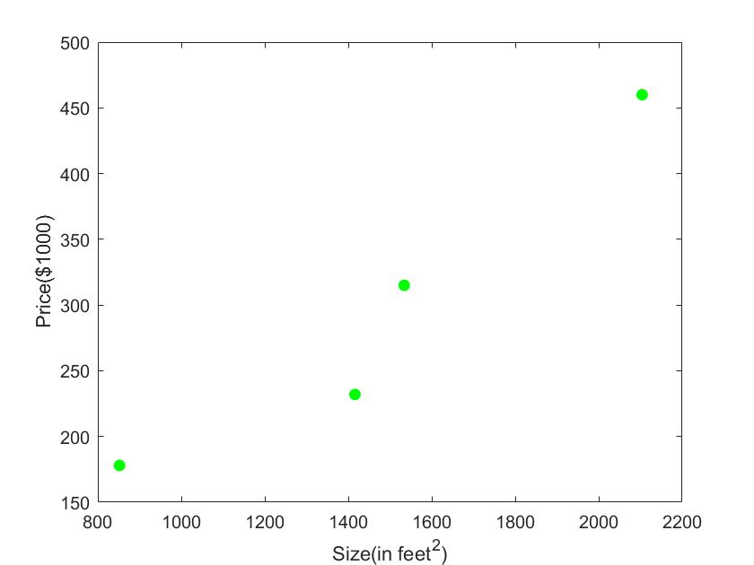
Plot between size and price of the house.
Now we need to generate a hypothesis function which is denoted by ‘h(x)’. It is a polynomial function that takes one or more parameters. For example:
![\[h(x)=\Theta_{1}*x+\Theta_{0}\] Or \[h(x)=\Theta _{2}*x^{2}+\Theta_{1}*x+\Theta _{0}\]](https://matlabhelper.com/wp-content/ql-cache/quicklatex.com-df57fc1869416247e217d63361b68521_l3.png)
It applies to all polynomial functions. For every input value (x), it predicts output using hypothesis function (h). The general form of hypothesis function is
![\[h_{i}(x)= \Theta _{1}*x+\Theta _{0}\]](https://matlabhelper.com/wp-content/ql-cache/quicklatex.com-09327ace28d11aefe7b6a3b040cd4228_l3.png)
Therefore ‘h’ is a vector of predicted values for an algorithm.
Our objective is to get the best possible line. The best possible line will be such that the average squared vertical distances of the scattered points from the line will be the least. Ideally, the line should pass through all the points of our training data set. In such a case, the value of cost function (J) will be zero. For the example mentioned above, Let’s consider
![\[\Theta_{1}=0.5\] and \[\Theta_{0}=0\]](https://matlabhelper.com/wp-content/ql-cache/quicklatex.com-7ca7f7406351faecac3ce9358e7292fd_l3.png)
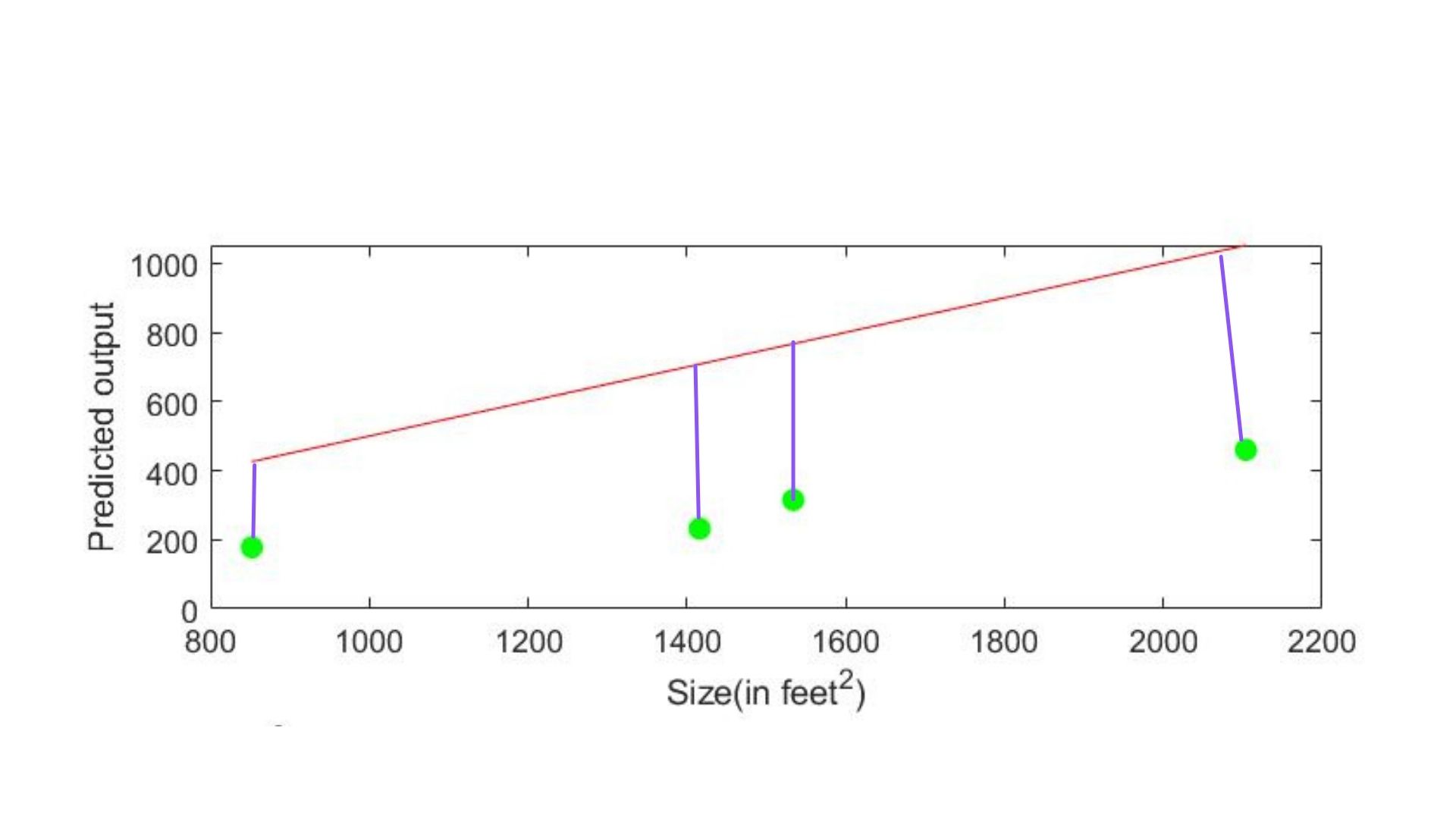
The plot of comparison between predicted output and actual output. The Red line shows the hypothesis function, and green circles are the actual output.
In the above figure, You can observe that the actual values (y, output of training data) and predicted values (h) are different and have some differences. So, To make the algorithm optimum, we need to reduce this difference during training. And this difference itself is called “Cost function”. The method used to reduce cost function is called “Gradient descent”.
Cost Function:
It is the average difference of all the results of the hypothesis (h) and the actual output (y). The cost function is denoted by “J”. This is also called as “Squared Error function” or “Mean square Error”. The mathematical equation is given by
![\[J(\Theta _{0},\Theta _{1})= 1/2*N \sum_{i=1}^{N}(h_{i}(x)-y_{i}))^{2}\]](https://matlabhelper.com/wp-content/ql-cache/quicklatex.com-a5b99f738ba66a4fbe4e4e9cb54774fa_l3.png)
Where N-->Number of training data.
h-->Predicted output
y-->Actual output
The mean is halved as a convenience for computation of the gradient descent as the derivative term of the square function will cancel out the halved term.
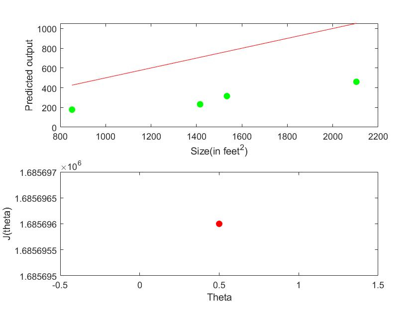
Cost function graph with theta=0.5.
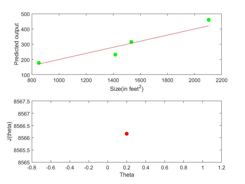
Cost function with theta=0.2
So from the above example, you understood that  and
and  are values that play an important role in prediction. Thus we have to improve this and values, such that the cost function reaches its optimal minimum. Therefore, the Gradient Descent algorithm is best to attain this feature.
Agriculture Quiz Contest - Q4'21
New Training Module on #ML
Course - Deep Learning
Be our Brand Representative
Gradient Descent:
It is an optimization approach for determining the values of a function’s parameters that minimizes a cost function. It is a derivative (the tangential line to the function) of the cost function. The slope of the tangent is the derivative at that point and it will give us a direction to move towards. We make steps down the cost function in the direction with the steepest descent. The size of each step is determined by the parameter  , which is called the “learning rate”.
For example, the distance between each “star” in the graph above represents a step determined by our parameter . A smaller would result in a smaller step, and a larger results in a larger step. The direction in which the step is taken is determined by the partial derivative of
![\[J(\Theta _{0},\Theta _{1})\]](https://matlabhelper.com/wp-content/ql-cache/quicklatex.com-b02bfa3815e885bb815ad561b42ef2c7_l3.png)
The gradient descent algorithm is given by:
Repeat until convergence:
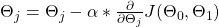
![\[\frac{\partial }{\partial \Theta _{j}}J(\Theta _{0},\Theta _{1})=1/N\sum_{i=1}^{N}(h(x)-y)*x\]](https://matlabhelper.com/wp-content/ql-cache/quicklatex.com-e60dc9131783c500526bb63faa504957_l3.png)
Therefore, Repeat until convergence:

Where j= 0,1 represents the feature index number
At each iteration j, one should simultaneously update the parameters  . Updating a specific parameter before calculating another one on the jth iteration would yield a wrong implementation.
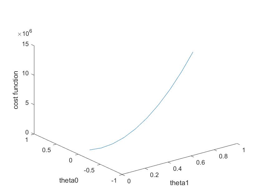
3D plot of Cost function to determine the optimal minimum (at 0.2,0) with respect to the cost function.
Here our objective is to converge the cost function to its minimum value. This convergence depends on the parameter “”.
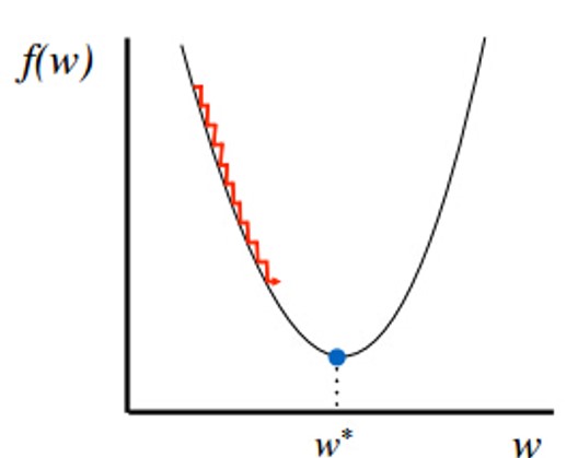
Plot of optimization of theta value when alpha is too small.
If “” is very small, gradient descent can be slow (It may take a long time to reach its minimum).
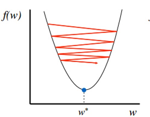
Plot of optimization of theta value when alpha is very large.
If “” is too large, gradient descent Can overshoot the minimum. It may fail to converge or even diverge.
MATLAB CODE:
% Author:Sneha G.K
% Topic :Cost Function in MATLAB
% Company: MATLAB Helper
% Website: https://MATLABHelper.com
%%%%%%%%%%%%%%%%%%%%%%%%%%%%%%%%%%%%%
% MATLAB code to find and improve parameter(theta value).
clc;
clear;
close all;
% Training data size of house(x) and price of house(y).
x=[2104 1416 1534 852];
y=[460 232 315 178];
%Theta value to be inserted in hypothesis function.
%Theta value can be 1x1 scalar or nx1 vector.
theta=input("Enter the theta1 value:");
N=length(y);
h=theta*x;%hypothesis fuction.
% Formula to find cost function.
Error=(h-y).^2;
J=(1/(2*N))*sum(Error);
disp(J);
% alpha to find gradient descent.
alpha=input("Enter alpha value:");
% Numbaer of times the parameters to be updated.
num_iter=input("Enter the number of times the parameter need to be updated:");
% The logic behind the gradient descent.
% If parameters are nx1 vector then another for loop has to inserted to
% updated every theta value.
for i=1:num_iter
Error=h-y;
delta=x'*Error;
theta=theta-(alpha/N)*sum(sum(delta));
h=theta*x;endError=(h-y).^2;
J=(1/(2*N))*sum(Error);
disp(J);
% display theta value
subplot(2,1,1);
plot(x,y,"ro","MarkerFacecolor","r");
hold on;
plot(x,h,"g-");
xlabel("Size(in feet^2)");
ylabel("Predicted value");
hold off;
subplot(2,1,2);
plot(theta,J,"bo","MarkerFacecolor","b");
Conclusion:
- The cost function is used to determine the quantity of error in prediction, which uses training data.
- Cost function plays an essential role in training the ML (Machine Learning) algorithm.
- A gradient descent algorithm is used to reduce the cost function for regression.
Loved our Blog Post? Give us your valuable feedback through comments!
Thank you for reading this blog. Do share this blog if you found it helpful. If you have any queries, post them in the comments or get in touch with us by emailing your questions to [email protected]. Follow us on LinkedIn, Facebook, and Subscribe to our YouTube Channel.
We will not share any code or resource which the author has not provided. If you are looking for free help, you can post your comment on the blog or video & wait for any community member to respond, which is not guaranteed. You can book Expert Help, a paid service, and get assistance in your requirement. If your timeline allows, we would recommend you to book the Research Assistance plan. If you want to get trained in MATLAB or Simulink, you may join one of our Training modules.
If you are ready for the paid service, share your requirement with necessary attachments & inform us about any Service preference along with the timeline. Once evaluated, we will revert to you with more details and the next suggested step.
Education is our future. MATLAB is our feature. Happy MATLABing!
If you find any bug or error on this or any other page on our website, please inform us & we will correct it.
Recommend
About Joyk
Aggregate valuable and interesting links.
Joyk means Joy of geeK