
9

Peaks, Peak Filtering, and Gray-Scale Weighted Centroids
source link: https://blogs.mathworks.com/steve/2021/10/04/peaks-peak-filtering-and-gray-scale-weighted-centroids/
Go to the source link to view the article. You can view the picture content, updated content and better typesetting reading experience. If the link is broken, please click the button below to view the snapshot at that time.

Peaks, Peak Filtering, and Gray-Scale Weighted Centroids » Steve on Image Processing with MATLAB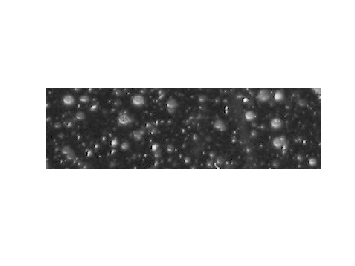


Today, I'm continuing my recent theme of thinking about peak-finding in images. When I wrote the first one (19-Aug-2021), I didn't realize it was going to turn into a series. This might be the last one—but no promises!
My previous post (17-Sep-2021) was based on 1-D examples. Today's post focuses on an image example (in 2-D), and it connects to using regionprops to compute gray-weighted centroids of peaks. I'll also throw in some 3-D surface visualization, just for fun. Here is today's image:
url = "https://blogs.mathworks.com/steve/files/snowflakes2.png";
A = imread(url);
imshow(A)
I'd like to see if we can focus algorithmically on these white blobby things (that's a technical term that I learned in engineering school). First, let's try computing the regional maxima.
A_regmax = imregionalmax(A);
imshow(A_regmax)
At first glance, that does not look like what I'm after. Let's find out what's going on here.
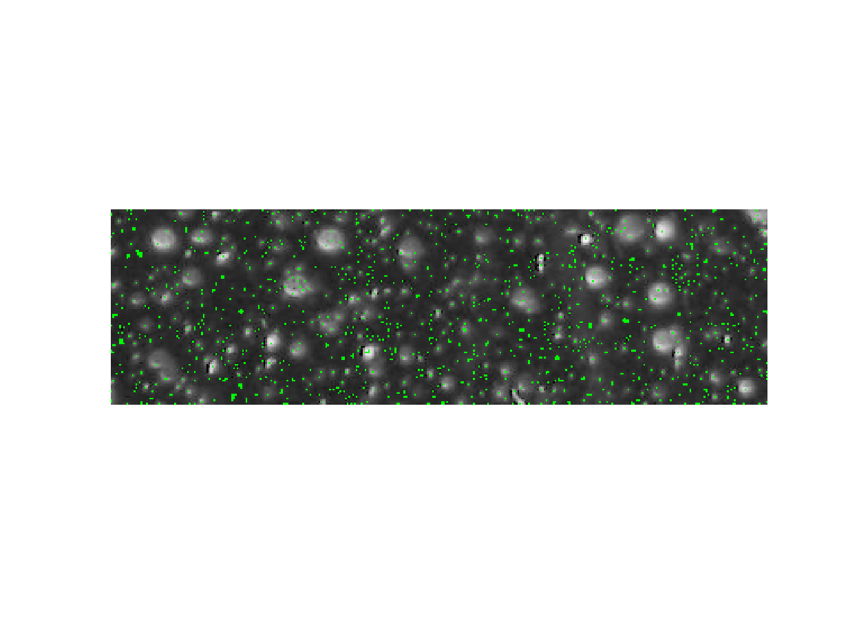
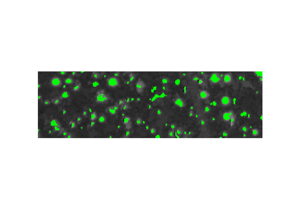
A_regmax_overlay = imoverlay(A,A_regmax,"green");
imshow(A_regmax_overlay)
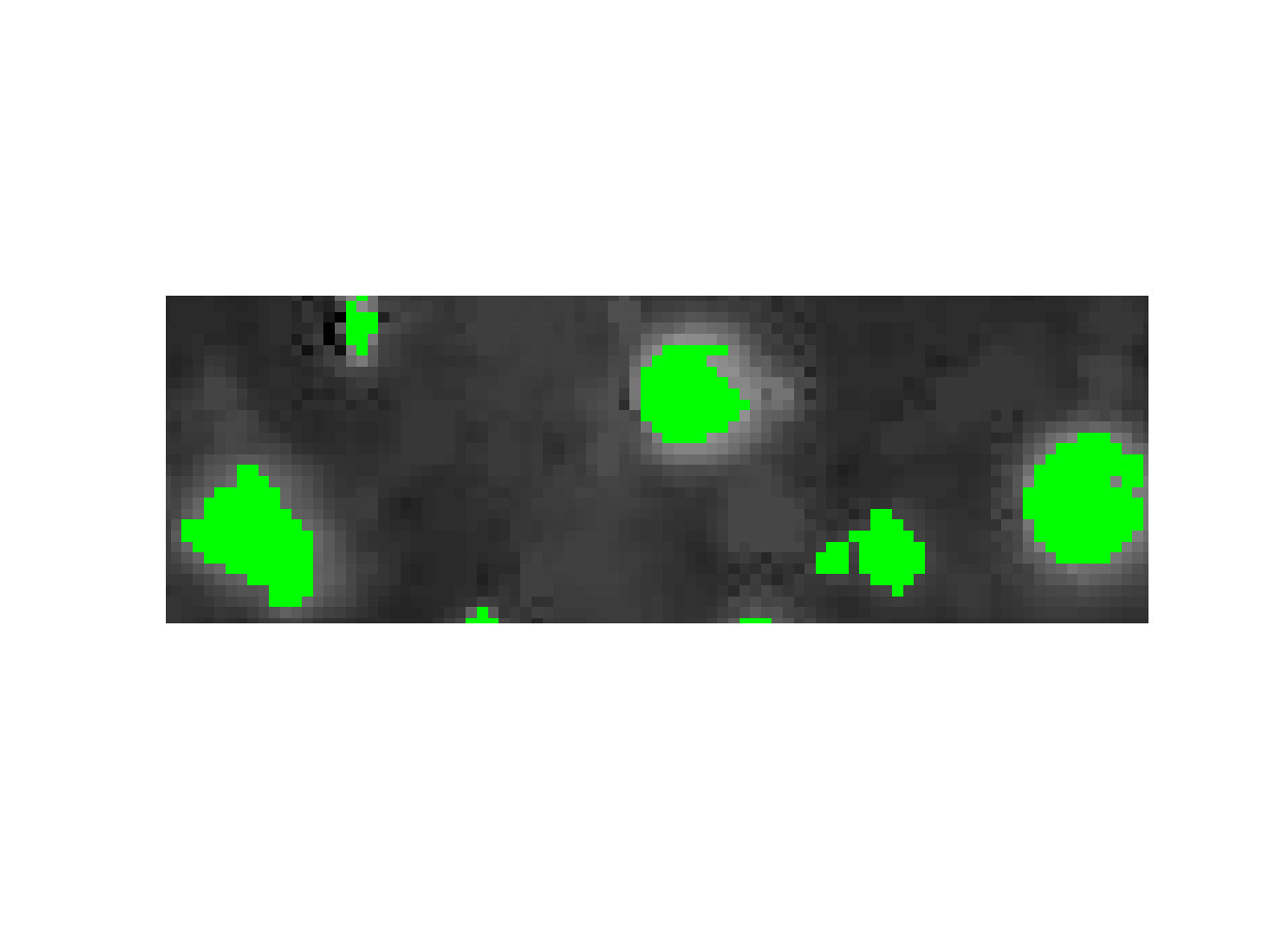
I want to look closely at one white blobby thing in particular.
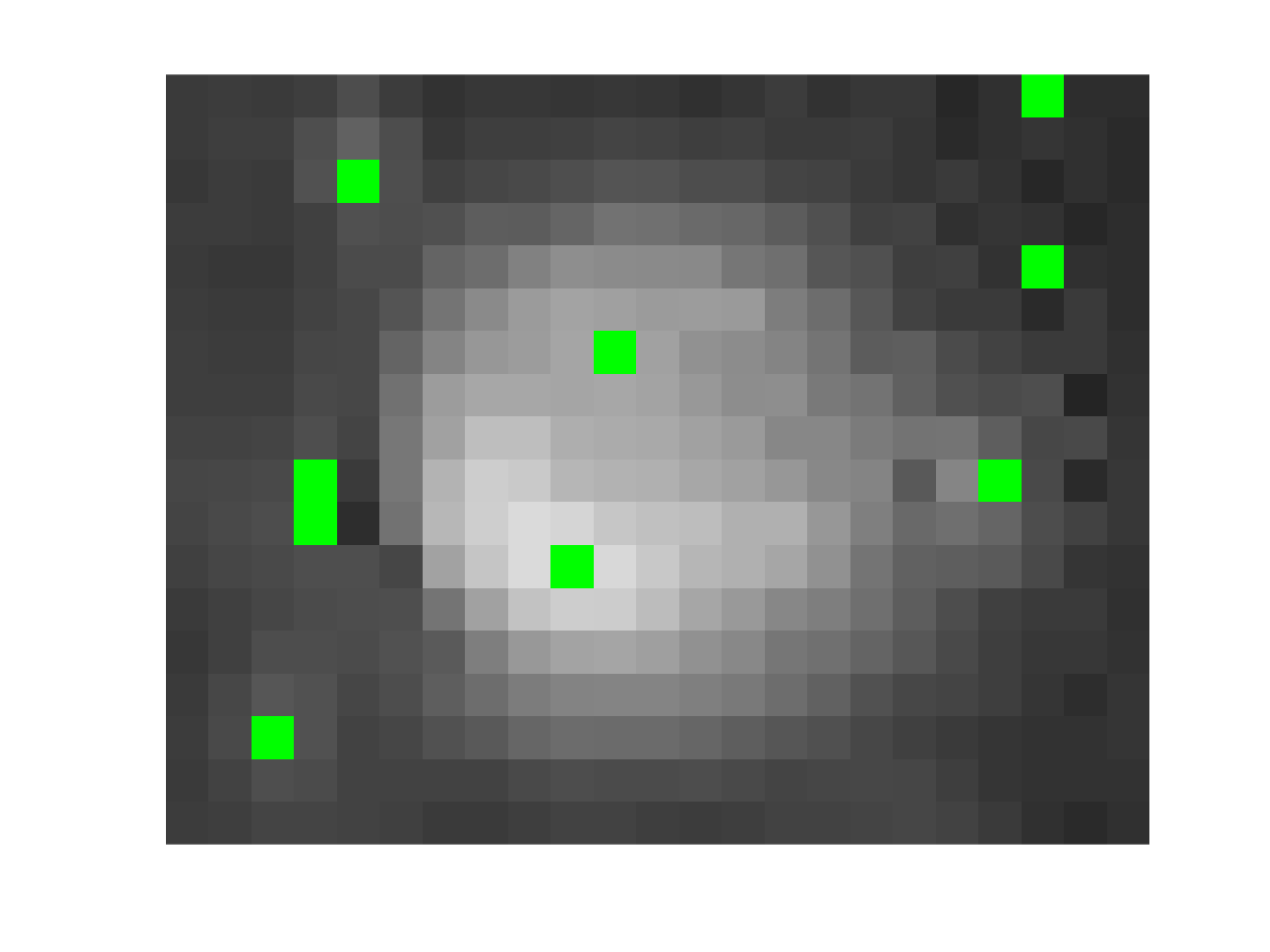
imshow(A_regmax_overlay(30:47,263:285,:))
One, or maybe two, of these locations looks like the kind of peak that we are interested in. What about the others? Let me show you two different ways to explore further. The first is with a 3-D visualization, where we treat the image pixel values as heights of a gray surface. The code below shows that surface, and then it displays the detected regional maxima as blue-and-yellow dots just above the surface.
figure
A_cropped = A(30:47,263:285);
A_regmax_cropped = A_regmax(30:47,263:285);
surf(A_cropped, EdgeColor = "none")
colormap("gray")
lighting gouraud
daspect([1 1 15])
[y,x,~] = find(A_regmax_cropped);
z = A_cropped(A_regmax_cropped);
hold on
plot3(x,y,z+1,LineStyle="none",Marker="o",...
MarkerEdgeColor="b",...
MarkerFaceColor="y")
xlabel("x")
ylabel("y")
set(gca,YDir = "reverse")
view(-35,45)
camlight
hold off
A second way is to go back to 2-D, but using an extremely zoomed-in view, with the actual pixel values superimposed on the individual pixels. To accomplish, I used the Image Viewer and the Pixel Region Tool. Below is a screen shot of the Pixel Region Tool. I have annotated the screen shot with the locations of the regional maxima.
With either technique, you can get the idea that several of these maxima locations are just small, uninteresting fluctuations.
As I discussed in the previous posts, you can use the h-maxima transform to filter out these small peaks.
h = 75;
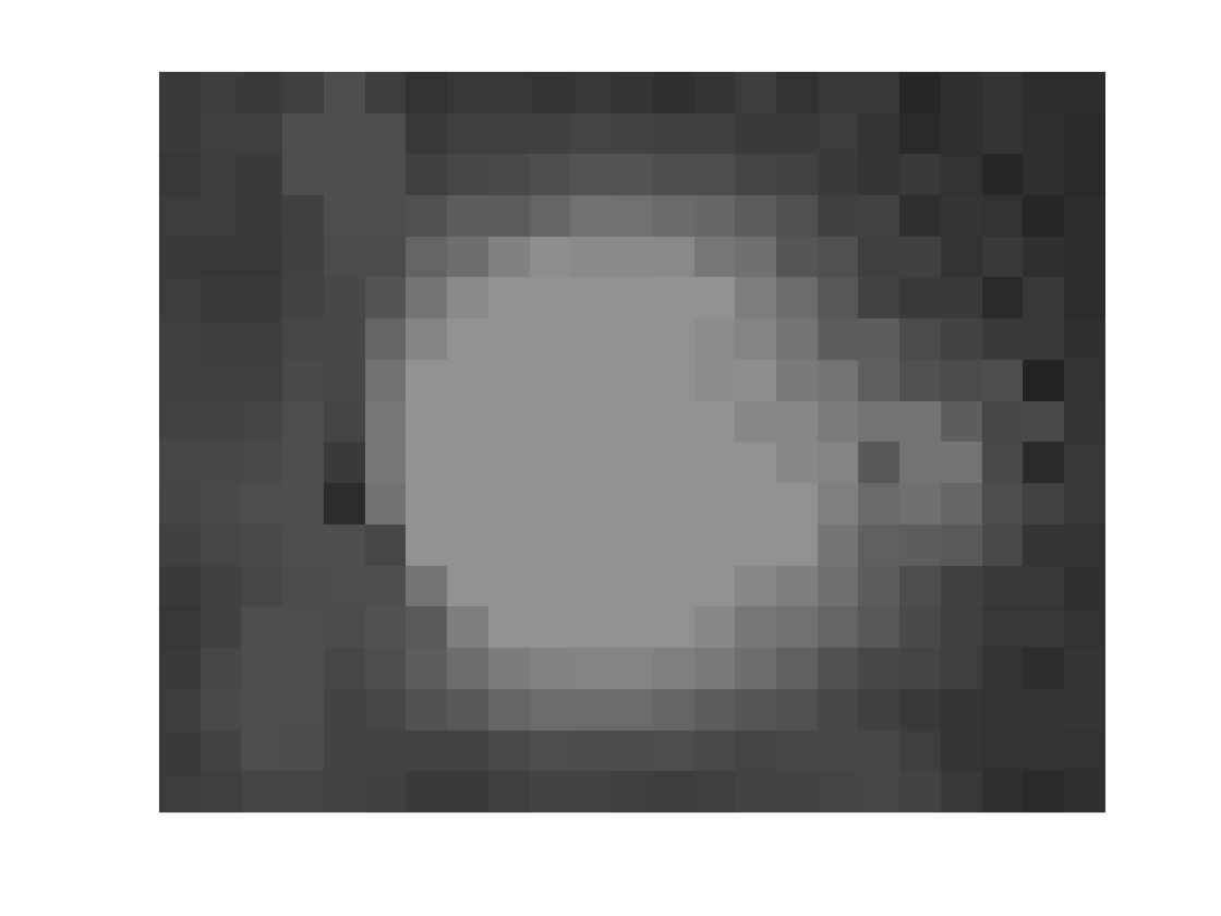
B = imhmax(A,h);
imshow(B(30:47,263:285))
B_regmax = imregionalmax(B);
imshow(B_regmax(30:47,263:285))
B_regmax_overlay = imoverlay(B,B_regmax,"green");
imshow(B_regmax_overlay)
axis([225 315 30 60])
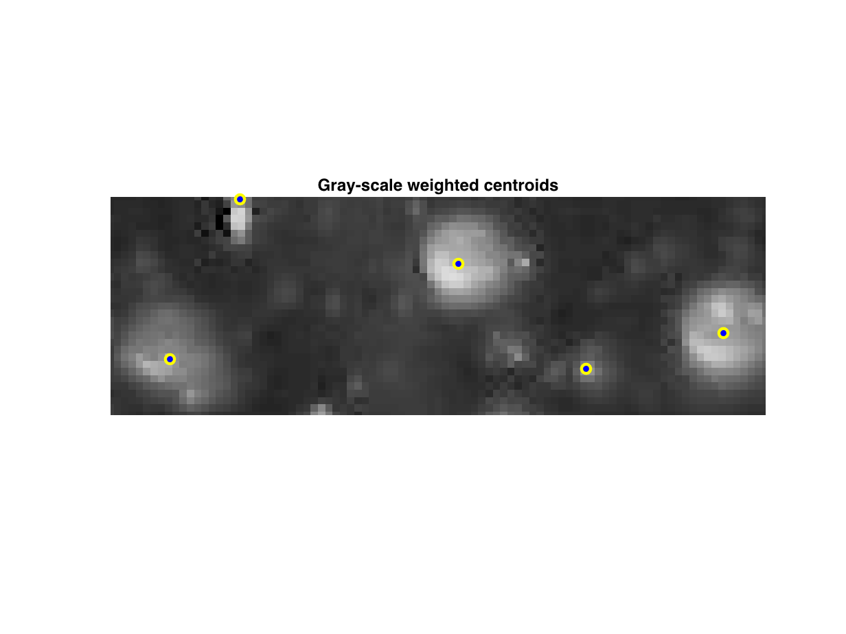
I want to finish up with a connection to the regionprops function. This function is used most often with a binary image input, and it computes various geometries properties of objects (connected components) in the binary image. But you can also provide a gray-scale image at the same time. With that additional info, you can compute other properties. Here, I am interested in the weighted centroids of the various detected peaks. The original image pixel values will be used as the weights. Here's how to do it:
props = regionprops("table",B_regmax,A,"WeightedCentroid")
props = 99×1 table
WeightedCentroid11.670224.613922.494843.359631.423997.7269414.581352.3127520.5567100.2771628.566389.2373729.977318.0773831.173150.3474941.20622.77181045.164539.64001144.122225.33521243.909867.87861344.8320103.42891450.909116.5648⋮
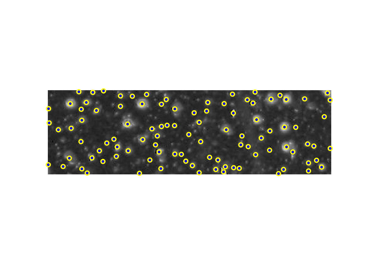
And here's one way to visualize the results:
imshow(A)
hold on
plot(props.WeightedCentroid(:,1),props.WeightedCentroid(:,2),...
LineStyle="none", Marker="o", MarkerEdgeColor="y",...
MarkerFaceColor="b")
hold off
axis([225 315 30 60])
title("Gray-scale weighted centroids")
Recommend
About Joyk
Aggregate valuable and interesting links.
Joyk means Joy of geeK