What Exactly Is A Gaussian Blur?

Blurring is a commonly used visual effect when digitally editing photos and videos. One of the most common blurs used in these fields is the Gaussian blur. You may have used this tool thousands of times without ever giving it greater thought. After all, it does a nice job and does indeed make things blurrier.

Of course, we often like to dig deeper here at Hackaday, so here’s our crash course on what’s going on when you run a Gaussian blur operation.

It’s Math! It’s All Math.

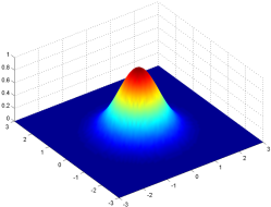A 2D Gaussian distribution shown in a 3D plot. Note the higher values towards the center, and growing smaller towards the outside in a bell curve shape.

Digital images are really just lots of numbers, so we can work with them mathematically. Each pixel that makes up a typical digital color image has three values- its intensity in red, green and blue. Of course, greyscale images consist of just a single value per pixel, representing its intensity on a scale from black to white, with greys in between.

Regardless of the image, whether color or greyscale, the basic principle of a Gaussian blur remains the same. Each pixel in the image we wish to blur is considered independently, and its value changed depending on its own value, and those of its surroundings, based on a filter matrix called a kernel.

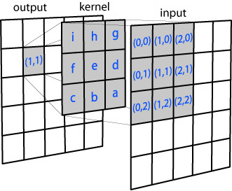This diagram shows the manner in which each pixel is processed. For a 3×3 kernel, the pixel of interest and all directly surrounding pixels are sampled. The kernel is then used to generate a new output pixel value based on a weighted average of the sampled pixels based on the Gaussian distribution.

The kernel consists of a rectangular array of numbers that follow a Gaussian distribution, AKA a normal distribution, or a bell curve. Our rectangular kernel consists of values that are higher in the middle and drop off towards the outer edges of the square array, like the height of a bell curve in two dimensions. The kernel corresponds to the number of pixels we consider when blurring each individual pixel. Larger kernels spread the blur around a wider region, as each pixel is modified by more of its surrounding pixels.

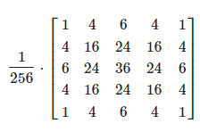A 5×5 Gaussian kernel. Note the external factor, which ensures that the total values all add up to 1. This avoids adding any intensity to the image, solely average the pixels without otherwise changing their intensity.

For each pixel to be subject to the blur operation, a rectangular section equal to the size of the kernel is taken around the pixel of interest itself. These surrounding pixel values are used to calculate a weighted average for the original pixel’s new value based on the Gaussian distribution in the kernel itself. Thanks to the distribution, the central pixel’s original value has the highest weight, so it doesn’t obliterate the image entirely.  Immediately neighboring pixels having the next highest influence on the new pixel, and so on. This local averaging smoothes out the pixel values, and that’s the blur.

Edge cases are straightforward too. Where an edge pixel is sampled, the otherwise non-existent surrounding pixels are either given the same value of their nearest neighbor, or given a value matching up with their mirror opposite pixel in the sampled area.

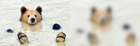Left, a source image. All the pixels inside the red border are the ones sampled to calculate the final value of the central red pixel when performing a Gaussian blur with a 7×7 kernel. Right, the result of the blur.

The same calculation is run for each pixel in the original image to be blurred, with the final output image made up of the pixel values calculated through the process. For grayscale images, it’s that simple. Color images can be done the same way, with the blur calculated separately for the red, green, and blue values of each pixel. Alternatively, you can specify the pixel values in some other color space and smooth them there.

Here we see an original image, and a version filtered with a Gaussian blur of kernel size three and kernel size ten. Note the increased blur as the kernel size increases. More pixels incorporated in the averaging results in more smoothing.

Of course, larger images require more calculations to deal with the greater number of pixels, and larger kernel sizes sample more surrounding pixels for each pixel of interest, and can thus take much longer to calculate. However, on modern computers, even blurring high-resolution images with huge kernel sizes can be done in the blink of an eye. Typically, however, it’s uncommon to use a kernel size larger than around 50 or so as things are usually already pretty blurry by that point.

The Gaussian blur is a great example of simple mathematics put to a powerful use in image processing. Now you know how it works on a fundamental level!