

Permutation tests and independent sorting of data
source link: https://blogs.sas.com/content/iml/2021/06/07/permutation-tests-sorting-data.html
Go to the source link to view the article. You can view the picture content, updated content and better typesetting reading experience. If the link is broken, please click the button below to view the snapshot at that time.
Permutation tests and independent sorting of data
0For many univariate statistics (mean, median, standard deviation, etc.), the order of the data is unimportant. If you sort univariate data, the mean and standard deviation do not change. However, you cannot sort an individual variable (independently) if you want to preserve its relationship with other variables. This statement is both obvious and profound. For example, the correlation between two variables X and Y depends on the (X,Y) pairs. If you sort Y independently and call the vector of sorted observations Z, then corr(X,Z) is typically not equal to corr(X,Y), even though Y and Z contain exactly the same data values.
This observation is the basis behind permutation tests for paired data values. In a permutation test, you repeatedly change the order of one of the variables independently of the other variable(s). The goal of a permutation test is to determine whether the original statistic is likely to be observed in a random pairing of the data values.
This article looks at how sorting one variable (independently of another) changes the correlation between two variables. You can use this technique to construct a new vector that has the same values (marginal distribution) but almost any correlation you want with the other vector.
A simple permutation: A sorted vector of values
The Sashelp.Class data set in SAS contains observations about the height, weight, age, and gender of 19 students. The Height and Weight variables are highly correlated (R = 0.88), as shown by the following call to PROC CORR in Base SAS:
data class;
set Sashelp.Class;
keep Height Weight;
run;

proc corr data=Class nosimple;
   var Height Weight;
run;
The output from PROC CORR computes the sample correlation between the Height and Weight variables as 0.88. The p-value is highly significant (p < .0001), which indicates that it would be rare to observe a statistic this large if the heights and weights were sampled randomly from an uncorrelated bivariate distribution.
Consider the following experiment: What happens if you sort the second variable and look at the correlation between the first variable and the sorted copy of the second variable? The following program runs the experiment twice, first with Weight sorted in increasing order, then again with Weight sorted in decreasing order:
/* sort only the second variable: First increasing order, then decreasing order */
proc sort data=Class(keep=Weight) out=Weight1(rename=(Weight=WeightIncr));
   by Weight;
run;
proc sort data=Class(keep=Weight) out=Weight2(rename=(Weight=WeightDecr));
   by descending Weight;
run;

/* add the sorted variables to the original data */
data Class2;
   merge Class Weight1 Weight2;
run;
/* what is the correlation between the first variable and permutations of the second variable? */
proc corr data=Class2 nosimple;
   var Weight WeightIncr WeightDecr;
   with Height;
run;
The output shows that the original variables were highly correlated. However, if you sort the weight variable in increasing order (WeightIncr), the sorted values have 0.06 correlation with the height values. This correlation is not significantly different from 0. Similarly, if you sort the Weight variable in decreasing order (WeightDecr), the sorted values have -0.09 correlation with the Height variable. This correlation is also not significantly different from 0.
It is not a surprise that permuting the values of the second variable changes the correlation with the first variable. After all, correlation measures how the variables co-vary. For the original data, large Height values tend to be paired with high Weight values. Same with the small values. Changing the order of the Weight variable destroys that relationship.
A permutation test for correlation
The experiment in the previous section demonstrates how a permutation test works for two variables. You start with pairs of observations and a statistic computed for those pairs (such as correlation). You want to know whether the statistic that you observe is significantly different than you would observe in random pairings of those same variables. To run a permutation test, you permute the values of the second variable, which results in a random pairing. You look at the distribution of values of the statistic when the values are paired randomly. You ask whether the original statistic is likely to have resulted from a random pairing of the values. If not, you reject the null hypothesis that the values are paired randomly.
You can use SAS/IML software and the RANPERM function to create a permutation test for correlation, as follows:
proc iml;
use Class2;
   read all var "Height" into X;
   read all var "Weight" into Y;
close;

start CorrCoeff(X, Y, method="Pearson");
   return ( corr(X||Y, method)[1,2] );   /* CORR returns a matrix; extract the correlation of the pair */
finish;

/* permutation test for correlation between two variables */
call randseed(12345);        /* set a random number seed */
B = 10000;                   /* total number of permutations */
PCorr = j(B, 1, .);          /* allocate vector for Pearson correlations */
PCorrObs = CorrCoeff(X, Y);  /* correlation for original data */
PCorr[1] = PCorrObs;
do i = 2 to B;
   permY = ranperm(Y)`;      /* permute order of Y */
   PCorr[i] = CorrCoeff(X, permY); /* correlation between X and permuted Y */
end;
The previous program computes a vector that has B=10,000 correlation coefficients. The first element in the vector is the observed correlation between X and Y. The remaining elements are the correlations between X and randomly permuted copies of Y. The following statement estimates the p-value for the null hypothesis that X and Y have zero correlation. The two-sided p-value is computed by counting the proportion of the permuted data vectors whose correlation with X is at least as great (in magnitude) as the observed statistic. You can also use a histogram to visualize the distribution of the correlation coefficient under the null hypothesis:
pVal = sum( abs(PCorr)>= abs(PCorrObs) ) / B;   /* proportion of permutations with extreme corr */
print pVal;

title "Permutation Test with H0:corr(X,Y)=0";
title2 "Distribution of Pearson Correlation (B=1000)";
refStmt = "refline " + char(PCorrObs) + " / axis=x lineattrs=(color=red);";
call histogram(PCorr) other=refStmt label="Pearson Correlation";
The graph and p-value give the same conclusion: It is unlikely that the observed statistic (0.88) would arise from a random pairing of the X and Y data values. The conclusion is that the observed correlation between X and Y is significantly different from zero. This conclusion agrees with the original PROC CORR analysis.
Find a vector that has a specified correlation with X
Every correlation coefficient in the previous histogram is the result of a permutation of Y. Each permutation has the same data values (marginal distribution) as Y, but a different correlation with X. An interesting side-effect of the permutation method is that you can specify a value of a correlation coefficient that is in the histogram (such as -0.3) and find a vector Z such that Z has the same marginal distribution as Y but corr(X,Z) is the specified value (approximately). The following SAS/IML statements use random permutations to find a data vector with those properties:
/* Note: We can find a vector Z that has the same
   values as Y but has (almost) any correlation we want!
   Choose the target correlation from the histogram, such as r=-0.3.
   Then find a vector Z that has the same values as Y but has corr(X,Z) = -0.3 */
targetR = -0.3;
isMatch = 0;
do i = 1 to B while(isMatch=0);   /* to avoid an infinite loop, limit search to B permutations */
   Z = ranperm(Y)`;          /* permute order of Y */
   r = CorrCoeff(X, Z);      /* correlation between X and permuted Y */
   isMatch = ( abs(r - targetR) < 0.01 );  /* is correlation close to target? */
end;

print r;
title "X versus Permutation of Y";
call scatter(X,Z);

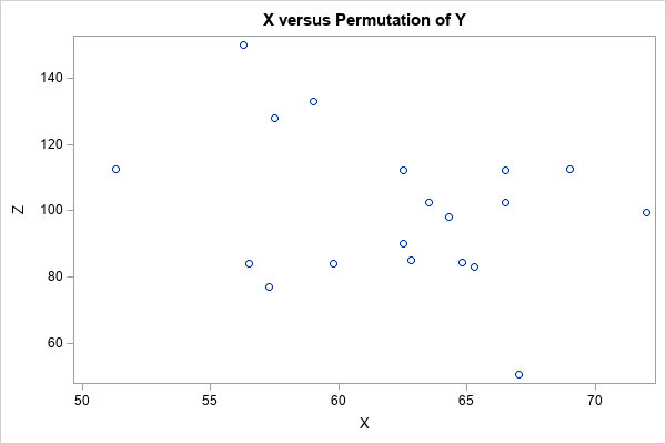
The scatter plot shows the bivariate distribution of X and Z, where Z has the same data values as Y, but the correlation with X is close to -0.3. You can choose a different target correlation (such as +0.25) and repeat the experiment. If you do not specify a target correlation that is too extreme (such as greater than 0.6), this method should find a data vector whose correlation with X is close to the specified value.
Notice that not all correlations are possible. There are at most n! permutations of Y, where n is the number of observations. Thus, a permutation test involves at most n! distinct correlation coefficients.
Summary and further reading
This article shows that permuting the data for one variable (Y) but not another (X) destroys the multivariate relationship between X and Y. This is the basis for permutations tests. In a permutation test, the null hypothesis is that the variables are not related. You test that hypothesis by using random permutations to generate fake data for Y that are unrelated to X. By comparing the observed statistic to the distribution of the statistic for the fake data, you can reject the null hypothesis.
An interesting side-effect of this process is that you can create a new vector of data values that has the same marginal distribution as the original data but has a different relationship with X. In a future article, I will show how to exploit this fact to generate simulated data that have a specified correlation.
For more information about permutation tests in SAS/IML, see
- My article about resampling and permutation tests in SAS, which uses a permutation test to examine the difference between two group means.
- John Vickery (2015) wrote an easy-to-read SAS Global Forum paper that provides an example of a permutation test for a matched-pair t-test.
Recommend
About Joyk
Aggregate valuable and interesting links.
Joyk means Joy of geeK