Today is March 14th, which is annually celebrated as Pi Day. Today's date, written as 3/14/16, represents the best five-digit approximation of pi.

On Pi Day, many people blog about how to approximate pi. This article uses a Monte Carlo simulation to estimate pi, in spite of the fact that "Monte Carlo methods are ... not a serious way to determine pi" (Ripley 2006, p. 197). However, this article demonstrates an important principle for statistical programmers that can be applied 365 days of the year. Namely, I describe two seemingly equivalent Monte Carlo methods that estimate pi and show that one method is better than the other "on average."

Monte Carlo estimates of pi

To compute Monte Carlo estimates of pi, you can use the function f(x) = sqrt(1 – x2). The graph of the function on the interval [0,1] is shown in the plot. The graph of the function forms a quarter circle of unit radius. The exact area under the curve is π / 4.

There are dozens of ways to use Monte Carlo simulation to estimate pi. Two common Monte Carlo techniques are described in an easy-to-read article by David Neal (The College Mathematics Journal, 1993).

The first is the "average value method," which uses random points in an interval to estimate the average value of a continuous function on the interval. The second is the "area method," which enables you to estimate areas by generating a uniform sample of points and counting how many fall into a planar region.

The average value method

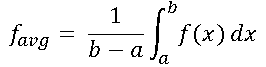
In calculus you learn that the average value of a continuous function f on the interval [a, b] is given by the following integral:

In particular, for f(x) = sqrt(1 – x2), the average value is π/4 because the integral is the area under the curve. In symbols,

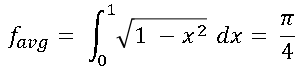
If you can estimate the left hand side of the equation, you can multiply the estimate by 4 to estimate pi.

Recall that if X is a uniformly distributed random variable on [0,1], then Y=f(X) is a random variable on [0,1] whose mean is favg. It is easy to estimate the mean of a random variable: you draw a random sample and compute the sample mean. The following SAS/IML program generates N=10,000 uniform variates in [0,1] and uses those values to estimate favg = E(f(X)). Multiplying that estimate by 4 gives an estimate for pi.

proc iml;
call randseed(3141592);       /* use digits of pi as a seed! */
N = 10000;
u = randfun(N, "Uniform");    /* U ~ U(0, 1) */
Y = sqrt(1 - u##2);
piEst1 = 4*mean(Y);           /* average value of a function */
print piEst1;

In spite of generating a random sample of size 10,000, the average value of this sample is only within 0.01 of the true value of pi. This doesn't seem to be a great estimate. Maybe this particular sample was "unlucky" due to random variation. You could generate a larger sample size (like a million values) to improve the estimate, but instead let's see how the area method performs.

The area method

Consider the same quarter circle as before. If you generate a 2-D point (an ordered pair) uniformly at random within the unit square, then the probability that the point is inside the quarter circle is equal to the ratio of the area of the quarter circle divided by the area of the unit square. That is, P(point inside circle) = Area(quarter circle) / Area(unit square) = π/4. It is easy to use a Monte Carlo simulation to estimate the probability P: generate N random points inside the unit square and count the proportion that fall in the quarter circle. The following statements continue the previous SAS/IML program:

u2 = randfun(N, "Uniform");   /* U2 ~ U(0, 1) */
isBelow = (u2 < Y);           /* binary indicator variable */
piEst2 = 4*mean(isBelow);     /* proportion of (u, u2) under curve */
print piEst2;

The estimate is within 0.0008 of the true value, which is closer than the value from the average value method.

Can we conclude from one simulation that the second method is better at estimating pi? Absolutely not! Longtime readers might remember the article "How to lie with a simulation" in which I intentionally chose a random number seed that produced a simulation that gave an uncharacteristic result. The article concluded by stating that when someone shows you the results of a simulation, you should ask to see several runs or to "determine the variance of the estimator so that you can compute the Monte Carlo standard error."

The variance of the Monte Carlo estimators

I confess: I experimented with many random number seeds before I found one that generated a sample for which the average value method produced a worse estimate than the area method. The truth is, the average values of the function usually give better estimates. To demonstrate this fact, the following statements generate 1,000 estimates for each method. For each set of estimates, the mean (called the Monte Carlo estimate) and the standard deviation (called the Monte Carlo standard error) are computed and displayed:

/* Use many Monte Carlo simulations to estimate the variance of each method */
NumSamples = 1000;
pi = j(NumSamples, 2);
do i = 1 to NumSamples;
   call randgen(u, "Uniform");         /*  U ~ U(0, 1) */
   call randgen(u2, "Uniform");        /* U2 ~ U(0, 1) */
   Y = sqrt(1 - u##2);
   pi[i,1] = 4*mean(Y);        /* Method 1: Avg function value */
   pi[i,2] = 4*mean(u2 < Y);   /* Method 2: proportion under curve */
end;
 
MCEst = mean(pi);              /* mean of estimates = MC est */
StdDev = std(pi);              /* std dev of estimates = MC std error */
print (MCEst//StdDev)[label="Comparison of Methods"
                      colname={"Avg Func" "Area"}
                      rowname={"MC Estimate" "MC StdErr"}];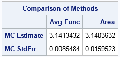

Now the truth is revealed! Both estimators provide a reasonable approximation of pi, but estimate from the average function method is better. More importantly, the standard error for the average function method is about half as large as for the area method.

You can visualize this result if you overlay the histograms of the 1,000 estimates for each method. The following graph shows the distribution of the two methods. The average function estimates are in red. The distribution is narrow and has a sharp peak at pi. In contrast, the area estimates are shown in blue. The distribution is wider and has a less pronounced peak at pi. The graph indicates that the average function method is more accurate because it has a smaller variance.

Estimating pi on Pi Day is fun, but this Pi Day experiment teaches an important lesson that is relevant 365 days of the year: If you have a choice between two ways to estimate some quantity, choose the method that has the smaller variance. For Monte Carlo estimation, a smaller variance means that you can use fewer Monte Carlo iterations to estimate the quantity. For the two Monte Carlo estimates of pi that are shown in this article, the method that computes the average function value is more accurate than the method that estimates area. Consequently, "on average" it will provide better estimates.