Galactic rotation curve and dark matter according to gravitomagnetism

Historically, the existence of dark matter has been postulated to resolve discrepancies between astrophysical observations and accepted theories of gravity. In particular, the measured rotation curve of galaxies provided much experimental support to the dark matter concept. However, most theories used to explain the rotation curve have been restricted to the Newtonian potential framework, disregarding the general relativistic corrections associated with mass currents. In this paper it is shown that the gravitomagnetic field produced by the currents modifies the galactic rotation curve, notably at large distances. The coupling between the Newtonian potential and the gravitomagnetic flux function results in a nonlinear differential equation that relates the rotation velocity to the mass density. The solution of this equation reproduces the galactic rotation curve without recourse to obscure dark matter components, as exemplified by three characteristic cases. A bi-dimensional model is developed that allows to estimate the total mass, the central mass density, and the overall shape of the galaxies, while fitting the measured luminosity and rotation curves. The effects attributed to dark matter can be simply explained by the gravitomagnetic field produced by the mass currents.

Mostly following the extensive work of Rubin et al. [1], measurements of the rotation of galaxies have shown that the rotation curves are essentially flat, with an initial steep increase and possible small velocity fluctuations related to spiral structures. The attempts to explain these observations used theoretical models derived on previous rotation studies of nebulae and galaxies. A summary of earlier work in this area has been given by de Vaucouleurs [2]. The first model for a spiral nebula was developed by Burbidge et al. [3] consisting in a series of concentric spheroidal shells of matter. In this way they obtained integral relations between the mass density and the rotational velocity. The system of shells was flattened by Brandt [4] to represent spiral galaxies as disk-like configurations, and improved by Brandt and Belton [5] to obtain the mass distribution in the form of a surface density. This method of calculation involves a double integral, so that it was further improved by Toomre [6] using alternative solutions based on Bessel functions, suited to the cylindrical geometry. Nordsiek [7] discussed the application of both the spheroid and disk methods in the analysis of rotation-curves, proposing simple mathematical models. Many of the previous spheroidal and disk models were reproduced by the Miyamoto–Nagai [8] potential-density pair, which provides a simple analytic solution to Poisson’s equation. One should mention that later Schorr [9] obtained an exact solution to the integral relating the mass distribution to the rotational velocity in the spheroid method.

Using different assumptions for the mass distribution and possible combinations of spheroids and disks, the above theoretical models failed to convincingly reproduce the observed flat rotation curves. The discrepancy between models and observations was more evident in the measurements of the rotation curve using the Doppler shifted 21  cm neutral hydrogen line (HI) outside the galactic central portion. Most of the visible mass is located in this central region. The only way to eliminate the discrepancy using the existent models was by the introduction of a halo of non-observable matter (dark matter) concentrated in the outer region of spiral galaxies. The role of this dark matter component was detailed by van Albada et al. [10] using improved HI data obtained by Begeman [11] for the extended rotation curve of NGC 3198. The main conclusion was that “the amount of dark matter inside the last point of the rotation curve, at 30  kpc, is at least 4 times larger than the amount of visible matter”. Subsequently, the methods of analysis became more sophisticated, but invariably introducing the dark matter component as detailed, for example, by Sofue et al. [12], Eadie and Harris [13], Sofue [14] and so many others. A detailed presentation of gravitational potential theory applied to several geometrical configurations of a large collection of stars, including the dark halo contribution, can be found in the book by Binney and Tremaine [15]. More recent models were advanced by Cooperstock and Tieu [16], Balasin and Grumiller [17], and Crosta et al. [18] considering general relativistic effects to describe the galactic dynamics. The relation between these papers and the present one is discussed later in this Introduction.

The motion of either stars or dust particles in a galaxy is determined by the gravitational interaction between masses only. The galactic system formed by a very large number of stars plus the surrounding gas can be approximated by a continuous mass distribution. This continuous fluid is essentially collisionless since binary encounters between stars are very rare (although long range encounters between passing stars determine the evolution of the system towards thermodynamic equilibrium on a very long time scale). Without binary encounters the interaction is described by collective Vlasov fields. Assuming steady-state the basic assumptions are established to describe the distributions of matter and of fluid velocity in a typical galaxy.

Now, most theories so far have been restricted to the Newtonian formulation or ad hoc modifications. They neglect relativistic corrections, which can significantly modify the rotation curve. Actually, at large distances the Lorentz force due to the gravitomagnetic field effectively controls the mass equilibrium balance in view of the decaying centrifugal force. The field produced by the large disk of mass currents basically acts as a gravitomagnetic brake against the gravitational attraction. Moreover, Newtonian theory leads to the condition that the centrifugal acceleration exactly balances the gravitational attraction in a circular orbit. But this condition can be strictly satisfied only for infinitesimally thin disks if pressure is neglected. As a further limitation, the thin disk approximation avoids the free boundary problem of galaxy equilibrium, when the shape of the galaxy is defined by a matching between the potential inside the fluid and the potential in vacuum.

Although filled with controversy, the studies of the galactic rotation via general relativity [16,17,18] reach the same basic conclusion of the present paper. Namely, the dragging effect of a gravitomagnetic component (time-space component of the metric) explains the flat rotation curve at large distances, without the recourse to dark matter. The main problem with the general relativistic models is the very limited number of exact solutions of the Einstein field equations. In particular, the study of galactic rotation relies in the use of the Kerr metric or suitable modifications, and its associated frame-dragging. In this context, it is very difficult to find self-consistent solutions relating the rotation velocity to the interior mass density distribution. This is illustrated by the fact that the general relativistic solutions reproduce, so far, the rotation curves in the distant region of a Kerr metric, without relating the derived mass density to the measured mass distributions, particularly near the axis of rotation where most of the mass is concentrated. This connection between rotation velocity, mass density and related brightness profiles is required by observational astronomy. The calculated motion in the general relativistic approach corresponds to the free-fall of test particles in the assumed metric, without consistently considering the effect of the large galactic mass density distribution on the metric. Actually, this is the same objection that can be made to the classical approach. Moreover, the free-boundary problem of the galactic shape also becomes highly intractable in general relativity. Interestingly, one should point out that the Gaia Collaboration effort [18, 19] allows to determine the motion in the weak local gravitational field resulting from the contribution of many relatively near mass concentrations. Fluid models, as used in the present paper, consider the mean motion of particles in the Vlasov-like collective gravitational field. The gravitoelectromagnetic weak field approximation to general relativity, used in the present paper, leads to a tractable self-consistent solution of the galactic rotation problem.

In summary, practically all the galactic rotation models so far are based on potential theory and the circular orbit concept in the Newtonian framework. Potential theory is entirely adequate when solving the Poisson equation for the gravitational potential. The problem arises when the circular velocity is estimated by a simple balance between the gravitational and centrifugal forces. A self-consistent calculation of the rotation velocity must take into account the gravitomagnetic field produced by the mass currents. In fact, the results of self-consistent calculations indicate a necessary change in the potential theory – circular orbit paradigm.

In the present article a new model for the rotation curve of galaxies is developed including the effects associated with mass currents. A set of equations that govern the motion of a weakly relativistic perfect fluid is introduced in Sect. 2. These equations are applied in Sect. 3 to the gravitational equilibrium of a pressureless, rotating fluid of dust in a form appropriate to the study of galaxies in steady-state. It is shown that the inclusion of the gravitomagnetic field clarifies some inconsistencies of the standard potential theory. Then, in Sect. 4, the equation that relates the velocity of rotation to the mass density distribution in equilibrium is developed. This equation is applied in Sect. 5 to the equilibrium of a compact object using the Miyamoto–Nagai [8] potential-density pair as solution of the Poisson equation. However, this solution is inadequate to describe the equilibrium of disk-like distributions, although illustrating the effects of the gravitomagnetic field. Therefore, an approximate bi-dimensional solution of Poisson’s equation is developed in Sect. 6 to describe the gravitational potential along the equatorial plane of disks of dust. This model is used in Sects. 7, 8 and 9 to adjust both the luminosity profiles and the rotation curves of galaxies NGC 1560, NGC 3198 and NGC 3115, respectively. Finally, Sect. 10 gives the conclusions. Appendix A demonstrates an important gravitomagnetic Cauchy invariant for a rotating fluid. Appendices B and C present details of the thin galactic disk model development. Appendix D describes the procedure to estimate the mass density in a galaxy from its surface-brightness profile.

The flow of a weakly relativistic perfect fluid of mass density \rho =nm, velocity {\varvec{v}} and pressure p in a self-consistent gravitoelectromagnetic (GEM) field is governed by the equation of continuity

by the momentum conservation (acceleration) equation

and by the GEM Maxwell’s equations for the field variables {\varvec{E}} and {\varvec{B}}:

where G is the gravitational constant and c denotes the velocity of light. In the present form the Lorentz force in the momentum conservation equation is limited to the linear velocity term, in accordance with the original gravitomagnetic theory developed by Thirring [20] and reviewed by Pfister [21]. The formulation of gravitoelectromagnetism and its effects were reviewed by Ruggiero and Tartaglia [22] and by Mashoon [23]. The linear approach to gravitoelectromagnetism is extensively adopted in the literature [24, 25]. An extended gravitoelectromagnetic theory was recently developed by the author of the present paper, describing the dynamics of a fully-relativistic perfect fluid in flat space in accordance with special relativity [26]. The connection between this extended theory and general relativity in its weak formulation was also accomplished [27]. Higher order terms in the velocity (higher then first order), are needed to describe many known general relativistic effects, such as the relativistic correction to the planetary precession of the perihelion and the production of gravitational waves. However, these effects are not important in the present context and the higher order terms can be safely disregarded. The paper is intended to develop a self-consistent model linking the Newtonian gravitational potential to the gravitomagnetic field. This link is obtained solving the equation of motion, coupled to Gauss’s law for the gravitational potential and Ampère’s law for the gravitomagnetic field. Ampère’s law has been used, for example, in the calculation of the Lense–Thirring effect, although not in a self-consistent form. The Lense–Thirring result, which was confirmed by measurements taken by Ciufolini and Pavlis [28] and later by the Gravity Probe B space experiment, as reported by Everitt et al. [29], is similar to calculating the magnetic field associated with a given current source (the rotating Earth in the Gravity Probe B case). However, the self-consistent solution must also consider how the mass currents are affected by the gravitomagnetic field. Note also that the orbit-orbit interactions entering the galactic equilibrium are much stronger than the spin-orbit interactions of the Lense–Thirring effect.

The total or convective derivative

gives the rate of change of a quantity moving instantaneously with the velocity {\varvec{v}}. It describes the advection by fluid motion. The gravitoelectromagnetic field variables are related to the scalar potential \phi and the vector potential {\varvec{A}} by

leading to the consistency relations:

Note that the vector potential {\varvec{A}} has been introduced without the factor 1/2 frequently used in gravitoelectromagnetism (the present definition simplifies the comparison with electromagnetic theory). The pressure p is related to the temperature T according to the isentropic flow condition ds/dt=0, which leads to the equation of state for a perfect fluid. Recall that the number density n is related to the temperature T by the perfect gas law p=nk_{B}T. The pressure term is here included for completeness, since it will be neglected from Sect. 3 onwards. In terms of the potentials the momentum conservation equation can be written as

In this Clebsch form the momentum conservation equation describes the evolution of the canonical momentum m\left( {\varvec{v}}+{\varvec{A}} \right) of a fluid element.

Note that Faraday’s law becomes entirely consistent in the gravitoelectromagnetic context if terms of higher order in the velocity of light are included, such as provided by a post-Minkowski theory [26, 27]. However, terms other than the first order term in the fluid velocity are needed in the Lorentz force only to obtain, for example, the relativistic correction to the perihelion precession, which is outside the scope of the present paper. This does not discard low-frequency inductive effects associated with Faraday’s law. The static field constraint in gravitomagnetism arises from imposing a total of four gauge-conditions on the metric tensor. Actually, only two conditions are allowed in an extended theory which includes gravitational waves. Moreover, in equilibrium the inductive or radiative effects related to Faraday’s law are irrelevant, so that in the present paper there is no need for higher order corrections in the equation of motion than the linear term provided by Thirring’s formulation in his third 1918 paper [20].

Note also that the electromagnetic field theory gives a result identical to the gravitoelectromagnetic field equations with the following analogies [30]

(2.8)

where {\varvec{E}}_{em} and {\varvec{B}}_{em} are the electromagnetic fields, \phi _{em} and {\varvec{A}}_{em} are the corresponding potentials, and the charge q in the Lorentz force is replaced by the mass m. With these analogies, the conservation equations describing the exchange of energy between the gravitoelectromagnetic field and matter can be obtained from a variational principle exactly in the same form as for the electromagnetic field.

Consider the equilibrium (\partial /\partial t\equiv 0) of a gravitationally confined dust configuration in rotation with negligible pressure (p\cong 0). Using the vector relation

the equilibrium is governed by the momentum conservation equation

and by the gravitoelectromagnetic laws of Gauss and Ampère, respectively,

In this way the equilibrium is described by eight variables formed by \rho , {\varvec{v}}, \phi and {\varvec{A}}. Note that Ampère’s law automatically satisfies the continuity equation in equilibrium

Since there are only seven equations one of the equilibrium profiles must be specified. In general, it is convenient to take the mass density distribution \rho as the independent variable.

Now, using the vector identity

the momentum conservation equation in equilibrium becomes

where \varvec{\omega }=\varvec{\nabla }\times {\varvec{v}} denotes the fluid vorticity. The scalar and vector products of the equilibrium equation with {\varvec{v}} give

Thus, in the direction of fluid motion the advection of specific kinetic energy is balanced by the Newtonian or gravitoelectric (GE) potential \phi . In the direction perpendicular to {\varvec{v}} the changes in the gravitoelectric potential and in the specific kinetic energy are balanced by both the fluid vorticity and the gravitomagnetic (GM) field {\varvec{B}}. If both vorticity \varvec{\omega } and the field {\varvec{B}} are neglected the above equations become a simple statement of the conservation of energy, leading to a singular irrotational vortex solution with finite velocity on axis. This solution is not acceptable, meaning that the flow is rotational (\varvec{\omega }\ne 0). But this raises the question of establishing rotational flow in an inviscid fluid. It turns out that the {\varvec{B}} field automatically leads to a rotational flow solution taking into account the Cauchy invariance of \left( \varvec{\omega }+{\varvec{B}}\right) /\rho (cf. Appendix A). In the absence of the gravitomagnetic field a fluid element that is initially in irrotational motion remains in this condition throughout the flow. But this condition is modified by the presence of the gravitomagnetic field. In this way a gravitomagnetic field introduces vorticity in an otherwise irrotational motion in an inviscid fluid, affecting mass accretion. The self-consistent {\varvec{B}} field constitutes a relativistic correction according to Ampère’s law.

As a further simplification, consider an equilibrium with fluid velocity in the azimuthal direction only, that is, {\varvec{v}} =v\widehat{\varvec{\varphi }}. Thus

so that the momentum conservation equations in equilibrium become

The gravitoelectric force is balanced by the fluid stress in the azimuthal direction, while the centrifugal and gravitomagnetic forces balance the gravitoelectric one in meridional planes. Note that the right-hand side of the meridional (poloidal) equilibrium equation shows the full dependence both on the vorticity and on the gravitomagnetic field. The first term on the right-hand side exactly cancels the second term on the left-hand side, indicating, as previously discussed, quite different solutions if vorticity and the gravitomagnetic field are or not taken into account. Furthermore, the gravitomagnetic field decreases the gravitational attraction in the latitudinal planes, provides the necessary equilibrium in the direction perpendicular to the equatorial plane, and confers vorticity to the fluid.

It follows that, in the case of a weakly relativistic rotational flow, that is, for \varvec{\omega }\ne 0 and {\varvec{B}}\ne 0 the equilibrium equations for a disk of dust in azimuthal motion are

The first equation above is automatically satisfied for an axisymmetric equilibrium. In this case the fluid equilibrium problem reduces to the two equations relating \phi , v and A_{\varphi } in the meridional plane. The set of equations is complete with the equations of Gauss and Ampère, which relate the gravitoelectric and gravitomagnetic potentials to the mass density and to the fluid velocity:

In axisymmetric cylindrical coordinates \left( R,\varphi ,Z\right) with

the poloidal equilibrium equations become

and, in terms of the gravitomagnetic flux function \psi =~RA_{\varphi },

The Ampère equation is in the form of the Grad–Shafranov equation for \psi . The poloidal flux function \psi can be eliminated using the equilibrium equations, so that the two-dimensional equilibrium problem reduces to a system of two second order differential equations relating \phi , \rho and v (the modified Grad–Shafranov equation involving \phi , \rho and v is manifestly nonlinear):

This shows that, although \phi is linearly related to \rho , the mass density can not be represented by a simple superposition of velocity components, and vice versa. Neglecting the effect of the gravitomagnetic mass currents in the right-hand side of the modified Grad–Shafranov equation (c\rightarrow \infty ), the solution of the one-dimensional model gives the balance condition between centrifugal and gravitational forces (neglecting \psi automatically leads to the one-dimensional constraint \partial /\partial Z\equiv 0)

This circular solution has been used in the galactic rotation curve analyzes so far, but is clearly inadequate in the light of relativistic effects.

Now, in the vacuum region (outside the volume V occupied by the galactic mass distribution) the gravitoelectric Newtonian potential is governed by Laplace’s equation

whose solution must satisfy the boundary condition at the surface S bounding the volume V. Since \phi is a solution of Laplace’s equation, \phi and \varvec{\nabla }\phi may not be independently specified over a given surface. It suffices to specify the Neumann condition on the surface S [31]:

where \sigma denotes an equivalent surface mass distribution defined by

Note that \widehat{{\varvec{n}}} is the normal to the surface, which points inward in the internal region and outwards in the external one. The gravitoelectric potential is continuous across the surface mass layer but the normal component of the gravitoelectric field suffers an increment:

Alternatively, the gravitoelectric potential in the vacuum region can be determined by the Dirichlet boundary condition specified by the value of \phi at the surface of the mass density distribution. This is true only if the surface S is known. In general, the unknown shape is determined by the Cauchy boundary condition (both Neumann and Dirichlet conditions). Inside the dust distribution \phi satisfies Poisson’s equation

Furthermore, \phi and \rho must satisfy the momentum equilibrium equation combined with Ampère’s equation (Grad–Shafranov equation) with {\varvec{v}} inside the fluid dust. The two-dimensional equilibrium constitutes a highly nonlinear free boundary problem defining the shape of the galactic disk.

It is instructive to write the equilibrium equations in terms of the vorticity and of the gravitoelectric and gravitomagnetic fields, respectively:

In cylindrical coordinates

The poloidal equilibrium equations for rotational motion become

clearly showing the role of the gravitomagnetic field in the confinement along the width of the disk of dust (axial balance). Along the radial direction the centrifugal force and the Lorentz force, which is associated to the gravitomagnetic field, balance the gravitoelectric attraction. Besides radial balance, the gravitomagnetic field is important in providing equilibrium along the direction perpendicular to the equatorial plane in a pressureless fluid, and in establishing a rotational flow. As will be shown from Sect. 5 onwards, it significantly modifies the rotation curve equilibrium solution, but first it is necessary to derive a workable equation which describes the velocity of rotation of dust in equilibrium.

The system of two differential equations (3.16) can be combined in the form

which depends only on the radial and vertical gradients of the gravitational potential. In general, the potential \phi \left( R,Z\right) is given in terms of the mass density distribution by inverting Gauss’s law (cf. Appendix B)

where K\left( m\right) denotes the complete elliptic integral of the first kind and m is the squared modulus

The radial and vertical gradients of \phi \left( R,Z\right) are given by

where E\left( m\right) denotes the complete elliptic integral of the second kind. Replacing these gradients in equation (4.1) one obtains a nonlinear, first-order partial differential equation for v\left( R,Z\right) in terms of the mass density \rho \left( R,Z\right) and its volume integrals. Since the rotation velocity is systematically measured along the galactic equatorial plane, one can take Z=0 so that, for a symmetric density profile,

where \beta =v\left( R,0\right) /c is the rotation velocity normalized to the velocity of light. Introducing the normalization radial distance R_{0} =1  kpc, one can define the normalized variables r=R/R_{0} and z=Z/R_{0}. The mass density \varrho =\rho /\rho _{0} is normalized with respect to the mass density at the origin \rho _{0}=\rho \left( 0,0\right) , and the gravitational potential \varphi =\phi /c^{2} is normalized by the velocity of light squared. Therefore,

where

and the squared modulus of the elliptic functions is

At this point it is convenient to introduce two dimensionless parameters (cf. Appendix C):

The parameter \lambda gives the ratio between the mass of a sphere of radius R_{0} and uniform density \rho _{0}, and the total mass M of the disk of dust. The equation for \beta ^{2} becomes

where

Defining the two functions of the mass density and its integral

the equation

can be identified as an Abel equation of the second kind for \beta ^{2} (the solution is obviously independent of the direction of rotation). This equation has no simple solution by quadrature, but can be easily solved by numerical methods. Since the origin is a singular point (\left. \beta \right| _{0}=0 and \left. \partial \beta /\partial r\right| _{0}=0), the integration must be carried out towards the origin for a given distant initial condition (similar to the Lane-Emden equation). The usual circular velocity assumption

leads to a constraint on the mass distribution along the equatorial plane

The mass distribution \varrho \left( r,0\right) forming f\left( r\right) must also satisfy equation (4.11) with \partial \varphi \left( r,0\right) /\partial r=\beta \left( r\right) ^{2}/r and \varphi \left( r,0\right) \sim \ln r if \beta \sim \,constant at large distances. This implies a singular one-dimensional solution with small (negligible) relativistic corrections. Removal of this singularity presumably leads to the introduction of dark matter for flat velocity profiles according to the standard (inadequate) circular velocity model.

The solution of the equation for the rotational velocity \beta \left( r,0\right) =\beta \left( r\right) in the equatorial plane (equivalent to Abel’s equation (4.13))

will be considered in this section for a spheroidal object described by the exact Miyamoto–Nagai [8] solution of Poisson’s equation (cf. Appendix C):

Inserting the expressions of g\left( r\right) =r\partial \varphi \left( r,0\right) /\partial r and f\left( r\right) =\left( 3\lambda r_{s}/2\right) \varrho \left( r,0\right) r^{2}, the equilibrium equation for the rotation velocity becomes, after some rearrangement,

The rotation velocity profile varies as a function of the normalized semi-axes a and b of the spheroid, and of the normalized Schwarzschild radius r_{s}. Since the origin is a singular point, as pointed out in the previous section, the initial value \beta \left( l_{\beta }\right) =\beta _{l} must be specified at some distant position l_{\beta } along the radial direction.

Fig. 1

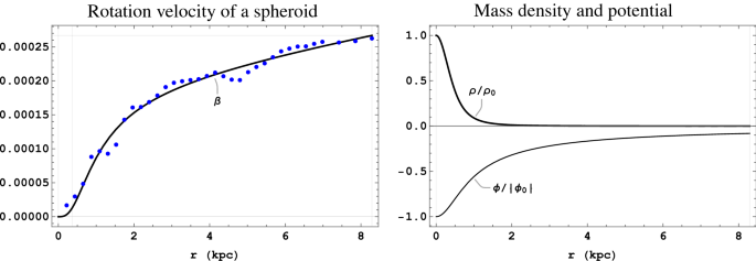
The left-hand side graphic shows the rotation curve of a compact spheroid fitted to the measured values for NGC 1560 (dots) as listed by Broeils [32]. The right-hand side graphic shows the normalized mass density and gravitational potential of the spheroid as given by the Miyamoto–Nagai [8] solution

Full size image

Fig. 2

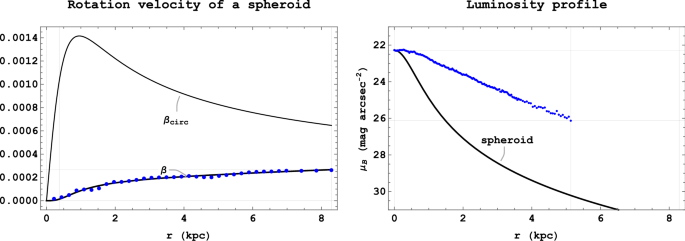
The left-hand side graphic shows a comparison between the fitted rotation curve and the standard definition of the circular velocity of a compact spheroid. The right-hand side graphic shows that the Miyamoto–Nagai solution fails to reproduce the luminosity profile of NGC 1560, as listed by Broeils [32] and represented by dots. The measured luminosity profile extends to the maximum radial distance 5.13 kpc

Full size image

Figure 1 shows the result of fitting a compact object to the observed rotation curve of the dwarf galaxy NGC 1560. [32, 33] The fitted parameters are: a=373  pc, b=300  pc and r_{s}=0.00701  pc, for l_{\beta }=8.29 kpc as the last point in the rotation curve data, where \beta _{l}\simeq 0.000267 corresponds to v\simeq 80  km/s. Note that the fitted (relatively large) normalized Schwarzschild radius corresponds to a total mass M\simeq 7.3\times 10^{10}M_{\odot } (M_{\odot }=1.9891\times 10^{30}   kg is the solar mass). The fitted semi-axes correspond to a massive, small, slightly oblate spheroidal object. Figure 1 also shows the normalized mass density and gravitational potentials described by the Miyamoto–Nagai solution. Figure 2 shows a comparison between the fitted solution and the velocity curve obtained from the potential according to the standard circular velocity definition. The circular velocity rises to large values in the transition region of the potential, but drops as expected by Kepler’s model in the low density region. On the contrary, the actual rotation velocity keeps rising well into the low density region, as described by the gravitomagnetic Abel equation. The gravitomagnetic field reduces the gravitational attraction and acts as a brake in the initial velocity rise (similarly, the relativistic correction to the planetary perihelion shift results from a balance between the gravitoelectric and gravitomagnetic forces). Although the compact object gives a reasonable fit to the rotation curve, it fails to reproduce the luminosity profile of NGC 1560, also shown in Fig. 2. The compact solution does not describe the equilibrium of large, disk-like objects, failing to reproduce its mass distribution and total mass. This failure arises because the Miyamoto–Nagai potential-density pair extends to infinity, without defining a galactic boundary. Unfortunately, the exact full solution of the gravitational potential of a disk of dust involves a complex two-dimensional free boundary problem as described in Sect. 3. Therefore, an approximate solution to the equilibrium of galactic disks will be developed in the next section.

A simplified, thin disk axisymmetric model for the gravitational potential will be derived in this section. In general, the gravitational potential is given in terms of the mass density distribution by means of a Green’s function (cf. equation (4.2) and Appendix B)

where K\left( m\right) denotes the complete elliptic integral of the first kind. Now, the integration over Z^{\prime } can be calculated using Laplace’s method for a thin disk mass density distribution of the form

Hence, the gravitational potential \phi \left( R,0\right) along the equatorial plane is given in terms of the mass density \rho \left( R,0\right) by the integration over R^{\prime }:

In terms of the normalized variables r=R/R_{0}, z=Z/R_{0}, \delta =\Delta /R_{0}, \varrho =\rho /\rho _{0} and \varphi =\phi /c^{2}, the previous expression becomes

The coefficient in front of the integral is expressed in terms of the dimensionless parameters already defined in Sect. 4:

The singularity for r=r^{\prime } in the integration over r^{\prime } can be circumvented by a change of variables from r^{\prime } to m (cf. Appendix B):

In the first integration branch, the integration variable 0\le m\le 1 runs from the origin (r^{\prime }=0) to the transition region m\lesssim 1 between the bulge and disk regions of the mass distribution. In the second integration branch, the integration variable 1\ge m\ge 0 runs along the disk region to infinity (r^{\prime }\rightarrow \infty ). The disk of dust has a maximum extension r_{\max } defined by \varrho \left( r,0\right) \simeq 0. To this maximum radial distance corresponds a minimum value m_{\min } of the integration variable in the second integration branch:

Therefore, the full integration over m can be divided along the two branches as follows:

The singularity r^{\prime }=r is restricted to the upper limit m=1 of the integrals, and can be avoided by taking m=1-\epsilon , where \epsilon is as small as required by the integration precision. The normalized radial gradient of the gravitational potential along the equatorial plane, \partial \varphi \left( r,0\right) /\partial r, is given by a similar expression presented in the Appendices B and C.

The simplified expressions of \varphi \left( r,0\right) and \partial \varphi \left( r,0\right) /\partial r can be used to define g\left( r\right) =r\partial \varphi \left( r,0\right) /\partial r in the left-hand side of equation (5.1). The mass density profile \varrho (r,0) can be estimated from the measured luminosity profile of the galactic disk. This same mass density defines the function f\left( r\right) =\left( 3\lambda r_{s}/2\right) \varrho \left( r,0\right) r^{2} in the right-hand side of equation (5.1). It remains to introduce a model for the galactic width \delta (r). This model is based on constant density contours of the Miyamoto–Nagai solution, as explained in the Appendix C, and amounts to solve the algebraic-integral equation for \delta (r):

where \lambda =\lambda \left( \ell ,a,b\right) is a normalizing coefficient (eigenvalue of the nonlinear algebraic-integral equation) calculated by

and the maximum radius of the disk is calculated by

The normalized geometrical parameters a and b correspond to the semi-axes of the Miyamoto–Nagai expression for the mass density, and the pre-defined range parameter \ell labels the density contours described by \delta \left( r\right) . The width \delta \left( r\right) defines the galactic shape and circumscribes a region containing a certain mass amount. Since the Miyamoto–Nagai solution extends to infinity, a value of \ell \simeq 3\sim 4 should contain practically all the total galactic mass M. The coefficient \lambda \left( \ell ,a,b\right) can be calculated by an iterative procedure described in the Appendix C. It must be evaluated for each set of values \ell , a and b while solving the Abel equation for \beta \left( r\right) . It turns out that the velocity profile is a function of the three free parameters a, b and r_{s} (assuming given \ell ). These parameters can be varied so that \beta \left( r\right) fits the observed galactic rotation curve, following the same procedure adopted in Sect. 5 for a spheroidal object, now constrained by a given mass density distribution along the equatorial plane. The nonlinear fitting procedure is quite demanding but produces the galactic shape \delta \left( r\right) as well as estimated values of the galactic mass M (given by r_{s}) and of the central density \rho _{0} (given by \lambda ). The solution of the algebraic-integral equation for \delta \left( r\right) corresponds to an approximate solution of the free-boundary galactic equilibrium problem. The luminosity profile is automatically fitted, since it serves as input for the mass density profile \rho \left( r,0\right) along the equatorial plane. If the potential-density pair with a definite boundary is known, the fitting procedure is carried out as exemplified in Sect. 5 for a spheroid, but with definite integration limits. In the next sections the case of NGC 1560 will be revaluated using the approximate thin disk model, followed by NGC 3198 and NGC 3115.

Fig. 3

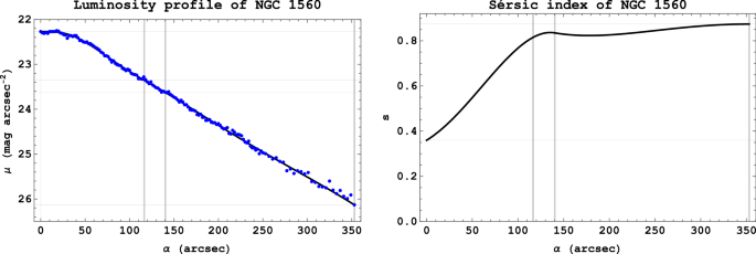
The line in the left-hand side graphic shows the adjusted luminosity profile of NGC 1560, and the dots correspond to the values listed by Broeils [32]. The right-hand side graphic shows the corresponding variable Sérsic index profile. The vertical lines in both graphics correspond to the effective half-angle \alpha _{\text {eff}} \cong 116.5 {\text {arcsec}} and to the transition point \alpha _{0}\cong 140.3 {\text {arcsec}} between the bulge and disk regions (r_{\text {eff}}\cong 1.69  kpc and r_{0}\cong 2.04  kpc). The profiles extend to the last measurement taken at l_{\rho }=5.13 kpc

Full size image

Fig. 4

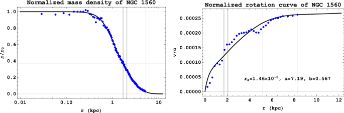
The line in the left-hand side graphic shows the mass density profile fitted to the observed luminosity profile of NGC 1560, represented by dots. The line in the right-hand side shows the rotation curve fitted to the experimental values listed by Broeils [32]. The thick vertical lines correspond to the effective half-radius r_{\text {eff}}\cong 1.69   kpc and to the transition point r_{0}\cong 2.04  kpc between the bulge and disk regions. The mass density at the radial position r_{\text {eff}} is equal to 1/e times the density at the origin

Full size image

Fig. 5

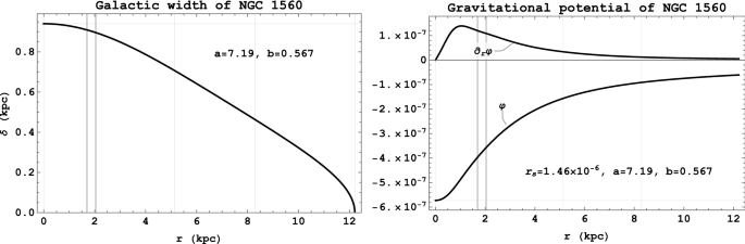
The left-hand side graphic shows the calculated width of NGC 1560, and the right-hand side the normalized gravitational potential and its radial derivative along the equatorial plane. The thick vertical lines correspond to the effective half-radius r_{\text {eff}}\cong 1.69   kpc and to the transition point r_{0}\cong 2.04  kpc between the bulge and disk regions

Full size image

The rotation curve of the dwarf galaxy NGC 1560 will be analyzed in this section, using the thin disk model developed in Sect. 6. The mass density is estimated from the surface-brightness profile measured by observational astronomy using an improved fitting procedure described in the Appendix D. Accordingly, Fig. 3 shows the luminosity and the Sérsic index profiles of NGC 1560 fitted by two series up to the fourth power in the bulge and disk regions. The adjusted numerical coefficients are (cf. Appendix D): \mu _{0}=22.27, \alpha _{\text {eff}}=116.5 (r_{\text {eff}}=1.69  kpc), \alpha _{0}=140.3 (r_{0}=2.04  kpc), s_{0}=0.360, b_{2}=0.0000344, b_{3}=-1.41\times 10^{-7}, b_{4}=-4.05\times 10^{-10}, d_{3}=-1.11\times 10^{-9}, and d_{4}=5.73\times 10^{-11} (\alpha _{e} =353.0, s_{e}=0.874, b_{1}=0.00245, and d_{2}=-3.22\times 10^{-6}). Using the variable Sérsic index profile, the calculated value of the absolute magnitude is M_{s}=-15.3, the total luminosity is L_{s} =1.02\times 10^{8}L_{\odot } and the apparent magnitude is m_{d}=12.1. The total luminosity is calculated up to the maximum galactic radius r_{max}=12.2 kpc that is estimated by the rotation velocity model described in the next paragraph. This value of the luminosity improves upon the value of the total luminosity given in the Appendix D, which is obtained assuming a luminosity profile with constant Sérsic index extending to infinity, according to the standard equation (D5).

The left-hand graphic in Fig. 4 shows the normalized mass density profile \varrho \left( r,0\right) obtained for NGC 1560 (the information in this figure is the same as displayed in Fig. 3). Now, \varrho \left( r,0\right) can be substituted in the equation (C18) for \partial \varphi \left( r,0\right) /\partial r and used to determine both the functions f\left( r\right) and g\left( r\right) in Abel’s equation (5.1). The solution of Abel’s equation depends on four parameters: the pre-defined range parameter \ell , the normalized Schwarzschild radius r_{s}, and the semi-axes parameters a and b. These parameters can be varied adjusting the solution of Abel’s equation to the measured rotation curve of NGC 1560, as shown in the right-hand side graphic of Fig. 4. The adjusted result is quite satisfactory, although a model with few parameters cannot reproduce the small oscillations in the rotation curve, which should be associated to oscillations in the density profile (this topic will be addressed in Sect. 8). Note that the mass density profile presents short range oscillations around 0.5 kpc and between about 4 and 5 kpc. The final set of adjusted parameters is: \ell =3, r_{s}=1.46\times 10^{-6}  kpc, a=7.19 kpc and b=0.567  kpc. The range parameter \ell =3 labels a constant density contour that contains approximately 1-\exp (\ell ^{2}/2)=0.989 of the total galactic mass M. This contour is shown in the left-hand graphic of Fig. 5 extending to a maximum radius r_{max} =12.2 kpc. Note that this corresponds to a very low density region according to the extended Sérsic profile, but large rotation velocity beyond the last point of measurement, at l_{\beta }=8.29  kpc. Figure 5 also shows the calculated gravitational potential. Finally, the total galactic mass estimated from the Schwarzschild radius is M\simeq 1.52\times 10^{10}M_{\odot } and the calculated coefficient \lambda =0.134 gives a central mass density \rho _{0}\simeq 3.31\times 10^{-20}  kg/m^{3}. The total mass-to-light ratio is \Upsilon =150\Upsilon _{\odot } and the total integration range, from the Schwarzschild radius to the maximum galactic extend, covers seven orders of magnitude.

The analysis of the spiral galaxy NGC 3198 [11, 34, 35] follows the same procedure established for NGC 1560, as presented in Sect. 7 and in the Appendix D. The observed brightness profile of NGC 3198 has a sharp peak near the origin, which decays to a not clearly defined disk region with large scale oscillations associated to the spiral structure. The main oscillations can be reasonably reproduced using a minimum of sixth order polynomials for s_{b} and s_{d} in Eq. (D17). The left-hand graphic in Fig. 6 shows a very good fit to the observed luminosity profile of NGC 3198, listed by Kent [34], using eighth order polynomials. The right-hand graphic shows the corresponding variable Sérsic index profile. The adjusted numerical coefficients are: \mu _{0}=19.49, \alpha _{\text {eff}}=22.4 (r_{\text {eff}}= 1.00  kpc), \alpha _{0}=154.0 (r_{0}=6.87  kpc), s_{0}=0.586, b_{2}=-0.000433, b_{3}=5.86\times 10^{-8}, b_{4}=3.29\times 10^{-9}, b_{5}=-1.06\times 10^{-11}, b_{6}=1.52\times 10^{-13}, b_{7}=2.90\times 10^{-15}, b_{8}=-1.75\times 10^{-17}, d_{3}=-4.96\times 10^{-7}, d_{4}=1.85\times 10^{-9}, d_{5}=1.07\times 10^{-11}, d_{6}=2.04\times 10^{-14}, d_{7}=-1.75\times 10^{-16}, and d_{8}=-1.20\times 10^{-18} (\alpha _{e}=316.8, s_{e}=1.49, b_{1}=0.0499, and d_{2}=0.0000181). Note that the matching point occurs after the main peak in the Sérsic profile. The calculated absolute magnitude considering the maximum radius r_{\text {max}}=30.7  kpc is M_{s}=-21.0, the total luminosity is L_{s}=1.93\times 10^{10}L_{\odot } and the apparent magnitude at d=9.2  Mpc is m_{d}=8.85.

Fig. 6

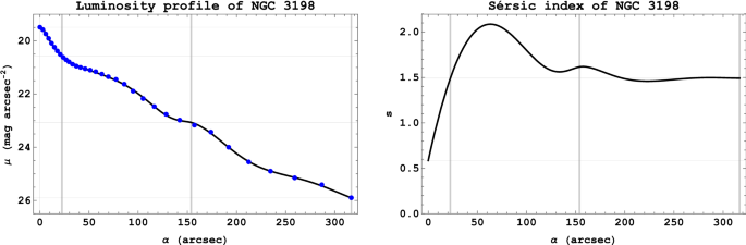
The left-hand side graphic shows the luminosity profile of NGC 3198 adjusted along the major galactic radius. The line in the graphic corresponds to the adjusted luminosity and the dots to the values listed by Kent [34]. The right-hand side graphic shows the adjustment obtained using two eighth-order polynomial approximations for the Sérsic index, as described in the text. The vertical lines in both graphics correspond to the effective half-angle \alpha _{\text {eff}}=22.4 arcsec and to the transition position \alpha _{0}=154.0 arcsec. The profiles extend to the last measurement taken at l_{\rho }=14.1  kpc

Full size image

Fig. 7

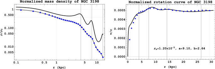
The thin line in the left-hand side graphic shows the mass density profile fitted to the observed luminosity profile of NGC 3198, listed by Kent [34] and represented by dots. The thick continuous line shows the mass density corrected for the high mass-to-light ratio population. The line in the right-hand side shows the rotation curve fitted to the experimental values listed by Begeman [11], represented by dots. The vertical lines in both graphics indicate the central positions of the spiral arms. The mass density profile extends to the last measurement taken at l_{\rho } =14.1  kpc. The last measured value of the rotation velocity lies at l_{\beta }=29.4 kpc

Full size image

Fig. 8

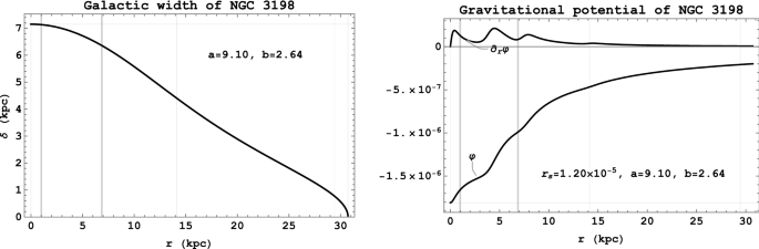
The left-hand side graphic shows the calculated shape of NGC 3198, and the right-hand side the normalized gravitational potential and its radial derivative along the equatorial plane. The vertical lines in both graphics correspond to the effective half-radius r_{\text {eff}}=1.00  kpc and to the transition position r_{0}=6.87  kpc

Full size image

The large scale oscillations in the luminosity profile are insufficient to fully describe the corresponding oscillations in the rotation velocity profile. These oscillations can be taken into account by the introduction of a population of high mass-to-light ratio spiral arms (at the intersections of the spiral arms). This population is tentatively represented by a function Y defined by a sum of n+1 Lorentzian (Cauchy) distributions

where r_{i} denotes the center of each Lorentzian and \gamma _{i} is the full width at half maximum. The center points are distributed according to a logarithmic spiral

where r_{\text {spiral}} is the initial radius. The amplitude of each Lorentzian component grows by a factor y_{i} distributed according to (taking y_{0}=0 gives an uniform mass-to-light distribution Y=1)

The amplitudes y_{i} correspond to the area of each Lorentzian distribution (one should point out that a distribution for non-negative variable, such as a the Lévy distribution, could give better results near the origin). The high mass-to-light ratio population is normalized so that Y\underset{r\rightarrow \infty }{\rightarrow }1. In the case of NGC 3198 the peaks can be approximately fitted by taking an initial radius r_{\text {spiral}}=4.0  kpc, a growth factor k_{\text {spiral}}=0.1, which corresponds to a polar slope angle \theta =\arctan k_{\text {spiral}}=5.71 {{}^\circ } , a constant width \gamma _{i}=\gamma _{0}=0.95  kpc, and an initial peak y_{0}=8.0 with \nu =1.4. The values of r_{\text {spiral}}, k_{\text {spiral}} and \gamma _{0} can be estimated by visual inspection of the fluctuations in the luminosity and rotation profiles. The values of y_{0} and \nu are obtained by fitting the rotation velocity profile, as described next.

The normalized mass density is given by the product of the high mass-to-light ratio population and the density obtained from the surface brightness distribution

where s\left( r\right) is the Sérsic profile adjusted to the luminosity:

The equilibrium solution shown in Figs. 7 and 8 corresponds to a normalized Schwarzschild radius r_{s}=1.20\times 10^{-5}   kpc, a major radius of the bulge a=9.10  kpc, a minor radius b=2.64  kpc, a range parameter \ell =3.0, a coefficient \lambda =0.00323 and a maximum radius r_{\text {max}}= 30.7  kpc. The calculated total mass of the galaxy is M=1.25\times 10^{11}M_{\odot }, the central density is \rho _{0} =6.54\times 10^{-21}  kg/m^{3}, and the total mass-to-light ratio is \Upsilon = 6.50\Upsilon _{\odot }. The large mass-to-light ratio ring currents associated with the spiral arms, and their gravitomagnetic field contributions, help to define the equilibrium and the fluctuations in the rotation curve. Without the ring currents the velocity profile is flat at large distance, but peaks near the origin. The additional gravitomagnetic field produced by the ring currents opposes the attractive Newtonian potential and introduces a dragging effect. Presumably, the relatively rapid rise of the calculated velocity curve is reduced by dispersion effects near the central position (this topic will be addressed again in Sect. 9). The integrated effect of short range oscillations near the origin can be simulated by the introduction of an equivalent pressure term in the equilibrium equation, but this requires further work. One must also take into account that NGC 3198 constitutes an elliptical spiral, so that the balance between the gravitoelectric force and the fluid stress in the azimuthal direction should be included in a detailed three-dimensional model. Nevertheless, the mass currents and associated gravitomagnetic fields are essential in establishing an equilibrium as described by Abel’s equation in two dimensions. The circular velocity approximation, if applied to the gravitational potential shown in Fig. 8, gives a strongly oscillating velocity distribution, peaked at r\simeq 5  kpc and decaying afterwards according to the Keplerian picture.

A reexamination of the NGC 1560 equilibrium indicates that the fit to the velocity curve can be slightly improved representing the small amplitude oscillations by a distributed high mass-to-light population with a broad maximum near r=4  kpc, but this addition obviously does not reproduce the short range velocity oscillations. The nonlinear Abel’s equation has two source functions depending on the mass density distribution: f(r) is directly proportional to \varrho (r) and g(r) depends on the integral of \varrho (r), so that these two contributions are not in phase and impact differently the rotation velocity. A consistent solution must include a detailed representation of the short and long range oscillations in the luminosity profile, including possible high mass-to-light ratio rings populations.

In this section the analysis of the lenticular (S0) galaxy NGC 3115 will be carried out [36,37,38,39,40]. The observed brightness has a very peaked profile near the origin, rapidly approaching an extended disk profile. The left-hand side of Fig. 9 shows the brightness profile of NGC 3115, which can be fitted by eighth- and seventh-order polynomials in the bulge and disk regions, respectively, as described in Sect. 7. The adjusted numerical coefficients are: \mu _{0}=15.21, \alpha _{\text {eff} }=1.88 (r_{\text {eff}}= 0.0911  kpc), \alpha _{0}=18.24 (r_{0}=0.884  kpc), s_{0}=0.845, b_{2}=-0.00291, b_{3} =-5.37\times 10^{-6}, b_{4}=-1.13\times 10^{-8}, b_{5}=2.84\times 10^{-10}, b_{6}=5.38\times 10^{-12}, b_{7}=7.62\times 10^{-15}, b_{8}=-1.07\times 10^{-16}, d_{3}=8.94\times 10^{-9}, d_{4}=-1.42\times 10^{-11}, d_{5}=-4.82\times 10^{-16}, d_{6}=2.04\times 10^{-17}, and d_{7} =-1.31\times 10^{-20} (\alpha _{e}=983.45, s_{e}=2.43, b_{1}=0.116, and d_{2}=-2.21\times 10^{-6}). The calculated absolute magnitude considering the maximum radius r_{\text {max}}=54.5  kpc is M_{s}=-21.9, the total luminosity is L_{s}=4.63\times 10^{10}L_{\odot } and the apparent magnitude at d=10.0  Mpc is m_{d}=8.08.

Fig. 9

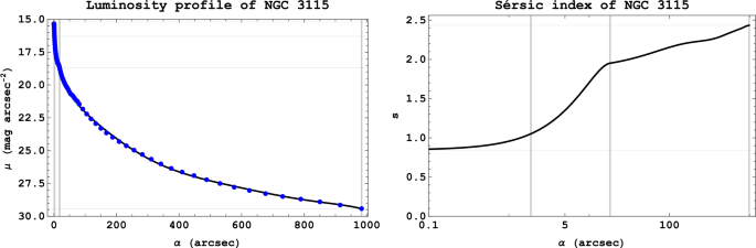
The line in the left-hand graphics shows the adjusted luminosity profile of NGC 3115, and the dots correspond to the values listed by Capaccioli [38]. The right-hand side graphic shows the adjustment obtained using eighth- and seventh-order polynomial approximations for the Sérsic index in the bulge and disk regions, respectively. The vertical lines in both graphics correspond to the effective half-angle \alpha _{\text {eff}}=1.88 arcsec and to the transition position \alpha _{0}=18.24 arcsec (r_{\text {eff}}= 0.0911  kpc and r_{0}=0.884  kpc). The profiles extend to the last measurement taken at l_{\rho }=47.7 kpc

Full size image

Fig. 10

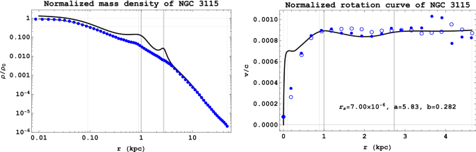
The thin line in the left-hand side graphic shows the mass density profile fitted to the observed luminosity profile of NGC 3115, listed by Capaccioli [38] and represented by dots. The thick continuous line shows the mass density corrected for the high mass-to-light ratio population. The line in the right-hand side shows the rotation curve fitted to the experimental values listed by Rubin et al. [37], represented by dots (the points correspond to the north following and the circles to the south preceding sides of the galaxy nucleus, respectively). The vertical lines in both graphics indicate the center positions of the two ring currents located near the inner edge of the disk region. The last measurement of the rotation curve is taken at l_{\beta }=4.64 kpc

Full size image

The equilibrium is maintained in part by two ring currents whose positions are barely indicated in the mass density and rotation curve profiles. These current rings can be represented taking two terms (i=0,1) in Eq. (8.1). The currents are located near the central region, at the inner edge of the disk region. Assuming k_{\text {spiral}}=0.16, r_{\text {spiral}}=1.0  kpc, \gamma _{0}=0.4  kpc, y_{0}=0.4 and \nu =0.3, the mass density is obtained multiplying the high mass-to-light ratio population Y(r) by the normalized mass density taken from the surface brightness distribution (initially assuming uniform mass-to-light ratio)

Fig. 11

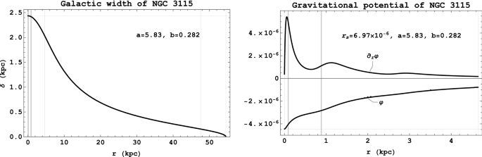
The left-hand side graphic shows the calculated shape of NGC 3115, and the right-hand side the normalized gravitational potential and its radial derivative along the equatorial plane. The vertical lines in both graphics correspond to the effective half-radius r_{\text {eff}}=0.0912  kpc and to the transition position r_{0}=0.884  kpc

Full size image

The equilibrium solution shown in Figs. 10 and 11 corresponds to a Schwarzschild radius r_{s}=6.97\times 10^{-6}  kpc, a major radius of the bulge a=5.83  kpc, a minor radius b=0.282  kpc, a range parameter \ell =4.3, a coefficient \lambda =0.432 and a maximum radius r_{\text {max}}=54.5  kpc. The large range parameter must be chosen in order to accommodate the very low mass densities at the maximum radius. The calculated total mass of the galaxy is M=7.28\times 10^{10}M_{\odot }, the central density is \rho _{0}=5.09\times 10^{-19}  kg/m^{3} and the total mass-to-light ratio is \Upsilon =1.57\Upsilon _{\odot }. The fit to the rotation curve is quite satisfactory, taking into account the dispersion of the data, excepting the rapid rise of the calculated values near the origin. It turns out that the improved kinematic data reported by Kormendy et al. [39], for NGC 3115, exhibits the same behavior displayed by the calculated rotation curve. According to Kormendy et al. [39], the rotation curve rises to approximately 165  km/s at 2  arcsec (r=0.0970  kpc), within a region of high dispersion. There is a plateau that extends towards the disk region, reaching 182  km/s at 7  arcsec (r=0.339  kpc). The central value of 295  km/s is attained at less than 20  arcsec (r=0.970  kpc). Figure 10 shows the same radial variation with a somewhat higher value of the velocity at the plateau. The calculated values are \beta \cong 0.00067 in the plateau and \beta \cong 0.00090 in the disk region. Nevertheless, the calculated values can be considered as effective velocity values in an essentially one-dimensional motion. The effective value v_{\text {eff}} is related to the average value {\overline{v}} by

so that the discrepancy between the calculated and measured velocities in the plateau can be accounted by a dispersion \sigma \cong 0.89 at 2  arcsec and \sigma \cong 0.67 at 7  arcsec, well within the dispersion values estimated from the measurements taken by Kormendy et al. [39]. The calculations also indicate that there is no need for a central black hole to explain the mass density peak and velocity dispersion near the origin.

Fig. 12

This figure corresponds to the information introduced in Fig. 10, the only difference being a small increase in the Schwarzschild radius, from r_{s}=6.97\times 10^{-6}  kpc to r_{s}=7.00\times 10^{-6}  kpc. Note the slight minimum in the rotation curve near 5  arcsec (r=0.24  kpc)

Full size image

Last, Fig. 12 shows the result of increasing the Schwarzschild radius by a small amount, from r_{s}=6.97\times 10^{-6}   kpc in Fig. 10 to r_{s} =7.00\times 10^{-6}  kpc. Although there is an imperceptible increase in the root-mean-square fitting error at the low velocity range, between the calculated values and the average values of the Rubin et al. [37] measurements, the new rotation curve has a slight minimum at \alpha \sim 5  arcsec, exactly as suggested by the high-resolution data of Kormendy et al. [39]. These results show the predictive power of the Abel equation for the rotation velocity, and the need of very accurate measurements of both the luminosity and the rotation velocity. With the small increase in the Schwarzschild radius, the calculated total mass of the galaxy is M=7.31\times 10^{10}M_{\odot }, the central density is \rho _{0} =5.11\times 10^{-19}  kg/m^{3} and the total mass-to-light ratio is \Upsilon =1.58\Upsilon _{\odot }. The modeling of galactic rotation curves will not be pursued further, since the main objective of the present paper is to show the importance of the gravitomagnetic field in explaining the rotation profile without recourse to dark matter.

A gravitomagnetic model was developed to calculate the rotation curve of galaxies without having recourse to dark matter components. One may say that the gravitomagnetic forces replace the dark matter effects. The self-consistent calculation of the rotation velocity takes into account relativistic corrections associated with the mass currents. The gravitomagnetic field produced by the currents plays four important roles in the self-consistent solution: (1) the Lorentz force associated to the gravitomagnetic field balances the Newtonian attractive force in the direction perpendicular to the equatorial plane in a pressureless equilibrium; (2) the gravitomagnetic field effects flow vorticity in an otherwise irrotational motion in an inviscid fluid; (3) the nonlinear coupling between the gravitomagnetic and Newtonian fields provides the mechanism for the transition between the rigid rotation flow near the origin and the constant speed flow near the edge; (4) at large distances the nearly constant gravitomagnetic Lorentz force added to the decaying centrifugal force balances the equally decaying gravitational attraction.

The balance between gravitoelectric, centrifugal, and gravitomagnetic forces in the moving fluid defines the mass distribution and affects the shape of the galactic disk. The actual shape is determined by the boundary condition matching the gravitoelectric potential and its gradient at the fluid-vacuum interface. Inside the dust equilibrium the gravitomagnetic field provides rotational flow in the absence of viscous forces. The Cauchy invariant demonstrated in the Appendix A indicates how the flow vorticity, gravitomagnetic field and mass density should distribute inside the galactic dust configuration during the time evolution.

The coupling between the gravitoelectric Newtonian potential and the gravitomagnetic flux function leads to a nonlinear relation between the rotation velocity and the mass density. The rotation velocity along the equatorial plane is governed by an Abel equation of the second kind, which reproduces the observations. Near the origin, where the gravitational field did not build up yet, the rotation curve shows a linear rise. Farther away from the origin the rotation speed shows a transition to a nearly constant value. At large distances the gravitomagnetic field is sufficiently intense to balance the decaying gravitational and centrifugal forces. Although the relativistic effects are weak (with a beta ratio of the order of 1/2000), the nonlinear coupling provides the mechanism that drives the transition in the rotation profile. This is similar to a soft phase transition, driven by weak perturbations, between asymptotic states. This transition between states should occur during the initial stages of formation of the galaxy, when the density rises at the origin and the potential well deepens. Near equilibrium the galaxy has been squeezed to its nearly disk-like shape bulging at the origin. This time evolution is a complex problem that requires much further study.

An approximate solution of the two-dimensional free boundary problem was developed based on constant density profiles defined by the Miyamoto–Nagai solution of the Poisson equation. This approximate solution was applied to three characteristic galaxies, showing that the observed rotation velocities can be reasonably reproduced while using the mass density profile, derived from the observed luminosity profiles, as input of the nonlinear Abel equation for the velocity. In this way, the rotation curves of NGC 1560, NGC 3198 and NGC 3115 were satisfactorily reproduced. In general, the additional contribution of high mass-to-light ring currents, and the associated gravitomagnetic field, is important in establishing equilibrium, notably in the case of spiral galaxies.

In conclusion, the galactic rotation curves were reproduced simply including the relativistic effects described by the gravitomagnetic field, without obscure dark matter components. The widely used one-dimensional circular-velocity thin disk model is clearly inadequate to find the galactic mass distribution. Possibly all calculations performed up-to-date using the thin disk circular velocity model must be reexamined, and the dark matter concept questioned, at least concerning the galactic rotation curves.

This manuscript has no associated data or the data will not be deposited. [Authors’ comment: This is a theoretical paper for which no data has been generated.]

This work was supported by a grant provided by the Programa de Capacitação Institucional: Diretoria de Pesquisa e Desenvolvimento/Comissão Nacional de Energia Nuclear (CNEN).

Affiliations

1. National Institute for Space Research, São José dos Campos, SP, 12227-010, Brazil

   G. O. Ludwig

2. National Commission for Nuclear Energy, Rio de Janeiro, RJ, 22294-900, Brazil

   G. O. Ludwig

Corresponding author

Correspondence to G. O. Ludwig.

Appendix A: A gravitomagnetic Cauchy invariant

The gravitomagnetic Cauchy invariant implies that the canonical vorticity divided by the mass density is the conserved quantity in a rotating fluid. In the weak relativistic limit the momentum conservation gives (the fully relativistic Cauchy invariant is demonstrated in reference [26])

This equation can be written in the form of a diffusion equation for the vorticity. Making use of the vector relation

the acceleration becomes

and the curl gives, using the continuity equation,

This leads to the vorticity diffusion equation

Now, assuming barotropic flow (in which the pressure p and the density \rho are directly related) the equation of motion gives, with the help of the gravitoelectromagnetic Faraday’s law,

It follows that the quantity \left( \varvec{\omega }+{\varvec{B}} \right) /\rho satisfies a modified vorticity equation

Introducing a change in the dependent variables as proposed by Serrin [41],

the vorticity equation becomes

Here \varvec{\nabla }_{0}{\varvec{r}}=\left| \partial {\varvec{r}} /\partial {\varvec{r}}_{0}\right| =\overline{\overline{{\varvec{J}}}} is the Jacobian dyadic of the transformation {\varvec{r}}= {\varvec{r}} \left( {\varvec{r}}_{0},t\right) from the Lagrangian {\varvec{r}} _{0} to the Eulerian {\varvec{r}} coordinates (\left| \overline{\overline{{\varvec{J}}}}\right| \ne 0 and \varvec{\nabla } _{0}\equiv \overline{\overline{{\varvec{J}}}}\cdot \varvec{\nabla }). The transformation {\varvec{r}}= {\varvec{r}}\left( {\varvec{r}} _{0},t\right) specifies the trajectory of a fluid element (or material particle). For fixed t, it determines the transformation of the fluid element from the initial position {\varvec{r}}_{0} to the position {\varvec{r}} at time t. Since

the vorticity equation reduces to

so that

Setting t=0

This result was obtained, for an incompressible fluid and without the gravitomagnetic field, by Cauchy [42] in 1815 and reviewed by Frisch and Villone [43]. In the absence of the gravitomagnetic field, this shows that a fluid element that is initially in irrotational motion remains in this condition throughout the flow. However, the modified vorticity equation shows that the gravitomagnetic field affects the vorticity distribution.

Appendix B: Green’s function for a thin galactic disk

In cylindrical coordinates with azimuthal symmetry, Poisson’s equation for the gravitational potential \phi takes the form

where \rho is the mass density distribution. The solution can be written in terms of the Green’s function {\mathcal {G}}(R,Z;R^{\prime },Z^{\prime })=1/\left| {\varvec{r}}-{\varvec{r}}^{\prime }\right| :

The Green’s function can be expressed in terms either of a toroidal function Q_{-1/2}\left( \chi \right) (Legendre function of the second kind, degree -1/2, order zero and type three) or a complete elliptic integral of the first kind K\left( m\right) [44,45,46]

where the argument 1\le \chi <\infty of the toroidal function is

and the squared modulus 0\le m\le 1 of the elliptic function is

so that

In terms of the elliptic integral

The radial and axial gradients of the Green’s function are given by

where E\left( m\right) denotes the complete elliptic integral of the second kind.

Consider the value of the potential along the equatorial plane (Z=0) for a vertically symmetric equilibrium

The potential at the field position \left( R,0\right) must be calculated by integration along the source position \left( R^{\prime },Z^{\prime }\right) . Changing variables, the integration along R^{\prime } can be divided in two branches along m:

where n=Z^{\prime }/R. Note that

where the upper and lower signs correspond to the first and second integration branches, respectively. In the first integration branch the variable 0\le m\lesssim 1 runs from zero to one in the radial range R^{\prime }/R\lesssim 1 (for Z^{\prime }\simeq 0) corresponding to the bulge of the density profile. In the second integration branch 1\gtrsim m>0 the radial range R^{\prime }/R\gtrsim 1 corresponds to the disk region with R^{\prime } extending to infinity. The transformed integral becomes

The upper limit in the integration over m has the limiting value (n=Z^{\prime }/R)

The above transformed integral expression of \phi \left( R,0\right) is exact. Now, for a thin disk the mass density distribution can be assumed of the form

In this approximation all cross-sections of the disk have the same form, but the characteristic width \Delta \left( R\right) varies with R. For small values of \Delta \left( R\right) the dominant term of the integration over Z^{\prime } is given by the Laplace approximation

In the original integration over R^{\prime } the thin disk approximation gives the simpler expression

but the transformed integration removes the Green’s function singularity by replacing the upper limit in the m integration by 1-\epsilon , where \epsilon can be taken as small as required by the precision of the calculation (the lower limit can also be replaced by \epsilon in order to avoid the divergence in the integrand for m\rightarrow 0).

In general, the integration along the disk branch ends at

where R_{\max } corresponds to the maximum extension of the disk defined by \rho \left( R_{\max },Z^{\prime }\right) \simeq 0. Along the equatorial plane the integration path is defined by Z^{\prime }=0 and

Therefore, for a thin disk the full integration over m can be divided along the two branches as follows

with the cut-off at the radial position along the equatorial plane \rho \left( R^{\prime },0\right) \simeq 0 explicitly taken into account. Similarly, the radial gradient of the gravitational potential is

Appendix C: A model for the galactic width

The mass density distribution \rho \left( R^{\prime },0\right) in the above integral expression of \phi \left( R,0\right) can be taken from the luminosity profile of the galaxy under consideration. However, a suitable model for the galactic width \Delta \left( R^{\prime }\right) must be developed to complete the description. This can be done considering the constant density contours defined by the Miyamoto and Nagai solution [8]

where A and B are the semi-axes of a spheroid of revolution. An exact solution of the Poisson equation gives the gravitational potential

where M is the total mass given by

Introducing the normalization radial distance R_{0}=1\,kpc, the Miyamoto and Nagai profile solution becomes

where all distances are normalized by R_{0} and the density \varrho =\rho /\rho _{0} is normalized by the value \rho _{0}=\rho \left( 0,0\right) at the center. One may introduce in the above expression a coefficient

which gives the ratio between the mass of a sphere of radius R_{0} and uniform density \rho _{0}, and the total mass M of the spheroidal distribution (\lambda measures the strength of the central density \rho _{0}). Hence,

The normalized potential \varphi =\phi /c^{2} becomes

where

is the normalized Schwarzschild radius of the spheroidal mass.

Although the Miyamoto and Nagai density profile extends to infinity, a galactic edge can be defined taking a constant density contour along the profile. According to the thin disk approximation (B14), one can define an edge such that \varrho \left( 0,\delta \left( 0\right) \right) on the vertical axis decreases by \ell characteristic widths with respect to the central density \varrho \left( 0,0\right) =1. In this way, the galactic shape is defined by \delta \left( r\right) along the profile and calculated by a root of the equation

where a is the major semi-axis in the radial direction and b the minor semi-axis in the vertical direction. According to the thin disk approximation it is assumed that a>3b (in general a\gg b). Exact analytic solution of this equation for \sqrt{b^{2}+\delta \left( r\right) ^{2}} is very difficult to achieve. It involves combination of roots 2, 4, 6 and 8 of a sixteenth order polynomial (roots 1, 3, 5 and 7 are negative and the remaining roots are complex). It is possible to obtain an approximate cubic solution for \delta \left( r\right) in Eq. (C9), but the numerical root-finding procedure can be easily implemented. Numerical calculation of \delta \left( r\right) as a function of r is straightforward for appropriate ranges of initial values a, b and \lambda \exp \left( -\ell ^{2}/2\right) . The range of possible values of \lambda is

so that r=0 and \delta \left( r\right) =0 at the upper value in the range. Taking \delta \left( r\right) =0, a given value of \lambda less than the upper limit defines the maximum value of the disk radius r=r_{\max } on the equatorial plane (r_{\max }\rightarrow \infty for \lambda \rightarrow 0):

Assuming b\ll a, this equation gives an estimate for the maximum radius of the galactic disk as a function of the relevant geometrical and physical parameters

This expression indicates that \ell can be identified as a range parameter. One would expect that a region described by the width \delta \left( r\right) calculated using equation (C9) contains approximately 39.3\%, 86.5\% and 98.9\% of the total galactic mass for \ell =1, 2 and 3, respectively. A region defined by \ell =4 contains practically all the total mass M (large values of \ell are required for very large disks containing a dim dust distribution at large distances).

Finally, note that \lambda cannot be specified independently, since its value is defined by the integral (C6), which, in the thin disk approximation, becomes

This constraint actually establishes the relation between a, b and the arbitrary normalization distance R_{0}. The value of \lambda can be determined by an iteration procedure as follows: \varvec{(1)} Take \lambda _{1}<1 and determine \delta \left( r\right) solving equation (C9) for given values of \ell , a and b; \varvec{(2)} Calculate r_{\max } solving equation (C11 ) for the same values of \ell , a, b and \lambda _{1}; \varvec{(3)} Calculate a new value \lambda _{2} by the integral (C13); \varvec{(4)} Compare the two values of \lambda _{2} and \lambda _{1} and stop the iteration if the error \left| \left( \lambda _{2}-\lambda _{1}\right) /\lambda _{1}\right| is less than the required precision (say 10^{-3}); \varvec{(5)} Define the new value \lambda _{1}=\left( \lambda _{1}+\lambda _{2}\right) /2 by the bisection method and repeat the iteration procedure until the required precision. As a result of this iteration, \lambda is determined as a function \lambda \left( \ell ,a,b\right) of \ell , a and b. A simple numerical procedure can be established so that \lambda \left( \ell ,a,b\right) is readily determined. In this way, one may consider the galactic width \delta \left( r\right) =\delta \left( \ell ,a,b,r\right) as given by a solution of (an algebraic–integral equation for \delta \left( r\right) )

and the maximum radius r_{\max }=r_{\max }\left( \ell ,a,b\right) of the disk by

Recall that the minimum value of m_{\min }=m_{\min }\left( \ell ,a,b,r\right) , which sets the radial extend in the disk region of the integrals for \phi \left( R,0\right) and \partial \phi \left( R,0\right) /\partial R defined in Appendix B, is given by

Introducing this lower (distant) limit, the normalized form the integral expressions for the gravitational potential and its radial gradient become:

Appendix D: Mass density estimate from surface-brightness profile

This appendix gives a brief presentation of the expressions used by observational astronomers to estimate the galactic luminosity and mass density, and the limitations of these simple definitions. In general, the mass density distribution along the equatorial plane of the galaxy can be evaluated from the measured surface-brightness profile, which can be approximated by the Sérsic profile for the flux density (in W/m^{2})

where s is the Sérsic index and R_{\text {eff}} is the half-luminosity radius, i.e., the radius that encloses half of the light, and b_{s} ^{-s}R_{\text {eff}} is the radius at which the central flux density F_{0} drops by e^{-1}. The coefficient b_{s} satisfies the relation

where \Gamma \left( 2s,b_{s}\right) and \Gamma \left( 2s\right) denote the incomplete and complete gamma functions, respectively. The coefficient b_{s} is given approximately by

The partial radiant flux (in W) is given by

so that the total radiant flux is (R\rightarrow \infty )

and the absolute magnitude is

where L_{10}=4\pi \left( 10\text {\, pc}\right) ^{2}F_{10} =3.0128\times 10^{28}  W is the standard radiant flux (luminosity) given in terms of the standard flux density F_{10}=2.518021002\times 10^{-8}   W/m^{2} (according to IAU resolution B2, 2015). The distance independent apparent magnitude is

The brightness profile is usually expressed in terms of the apparent magnitude in {\text {arcsec}}^{2}

where \alpha _{\text {eff}}=\left( 180\times 3600/\pi \right) b_{s} ^{-s}R_{\text {eff}}/d is the effective half-angle in {\text {arcsec}} and d is the distance to the galaxy. The apparent magnitude of the galaxy seen from Earth is

The de Vaucoulers’s profile for elliptical galaxies corresponds to s=4, while the simple exponential profile corresponds to s=1. Larger s gives light profiles concentrated in the central part, and at the same time higher surface brightness at large radial distances. These two profiles cannot be applied singly to represent the mass density \rho (r,0) because they have singular derivatives at the origin. Nevertheless, it is here proposed to construct a piecewise continuous profile defined by the juxtaposition of two Sérsic profiles:

This piecewise profile has continuous amplitude and derivative at R=R_{0} (not to be confounded with the normalization radius introduced in Sect. 4), and finite values at the origin if 0\le s_{1}<1 (the derivative vanishes at the origin if 0\le s_{1}<1). The profile is flat for s_{1}\gtrsim 0 and peaked for s_{1}\lesssim 1 (s_{1}=1/2 corresponds to a Gaussian profile near the origin). The piecewise profile for the apparent magnitude in {\text {arcsec}}^{2} becomes:

As an example, the surface brightness \mu _{B} of the dwarf galaxy NGC 1560 analyzed in Sect. 7 can be adjusted to the observed values listed by Broeils [32] by taking \mu _{0}=22.28, \alpha _{0}=61.46  {\text {arcsec}}, s_{1}=0.435, \alpha _{1}=99.05 {\text {arcsec}} and s_{2}=1.144 in the above expression. This approximation indicates a transition from a nearly Gaussian to a nearly exponential profile, and can be used to estimate the basic galactic parameters. The projected distances along the equatorial plane are calculated in terms of the angles of observation by r=d\left( \pi /\left( 180\times 3600\right) \right) \alpha . The calculated absolute magnitude is M_{s}=-16.5, the total luminosity is L_{s}=3.06\times 10^{8}L_{\odot } and, assuming a distance to the galaxy d=3.0\text {\, Mpc}, the apparent magnitude is m_{d}=10.9 (L_{\odot }=3.828\times 10^{26}   W is the solar luminosity).

The normalized mass density profile can be obtained directly from the adjusted luminosity profile by taking

where r_{0}=d\left( \pi /\left( 180\times 3600\right) \right) \alpha _{0} and r_{1}=d\left( \pi /\left( 180\times 3600\right) \right) \alpha _{1}. Assuming uniform mass-to-light ratio Y, one can take Y=1 without modifying the mass density profile. Although satisfactory for macroscopic estimates, the piecewise continuous approximation of the mass density is, in general, not satisfactory for detailed rotation velocity calculations since the Sérsic index in the above representation makes a discontinuous transition from the constant value s_{1} in the bulge region, 0\le r\le r_{0}, to the constant value s_{2} in the disk region, r>r_{0}. This limitation can be circumvented adopting a piecewise continuous representation for the Sérsic index instead

where s_{b}\left( \alpha \right) and s_{d}\left( \alpha \right) are power series defined separately in the bulge and in the disk regions:

The coefficients b_{i} and d_{j} can be chosen so that s_{b}\left( 0\right) =s_{0} and s_{d}\left( \alpha _{e}\right) =s_{e}, where s_{0} and s_{e} are the initial and final values of the Sérsic index in the range of measured values. Furthermore, the values and first derivatives of the index must be continuous at the transition point \alpha _{0} between the bulge and the disk:

Finally, it is required that the radial derivative of the index vanishes at the endpoint \alpha _{e} (this requirement is not essential, but it is convenient to have a flat index in extending the index beyond the last measurement point)

The final result can be written as follows:

where

According to Eq. (D8), the Sérsic index is given in terms of the apparent magnitude \mu \left( \alpha \right) at the angular position \alpha in {\text {arcsec}} by

This provides a relation between the index s_{e} at the last measured angular position \alpha _{e}, and the effective half-angle

Furthermore,

In this way, the values of \mu _{0}, \alpha _{\text {eff}}, \alpha _{0}, s_{0} and the power series coefficients b_{i} and d_{j} can be determined using a least squares method to fit s\left( \alpha \right) to the measured brightness profile. It is convenient to specify the initial value \mu _{0}, based on measurements, adjusting \alpha _{\text {eff}}, \alpha _{0} and the power series coefficients independently. The relation (D21) can be used to verify the consistency of the adjusted results. In terms of the radial position r one can simply replace \alpha by \left( 180\times 3600/\pi \right) r/d.

Open Access This article is licensed under a Creative Commons Attribution 4.0 International License, which permits use, sharing, adaptation, distribution and reproduction in any medium or format, as long as you give appropriate credit to the original author(s) and the source, provide a link to the Creative Commons licence, and indicate if changes were made. The images or other third party material in this article are included in the article’s Creative Commons licence, unless indicated otherwise in a credit line to the material. If material is not included in the article’s Creative Commons licence and your intended use is not permitted by statutory regulation or exceeds the permitted use, you will need to obtain permission directly from the copyright holder. To view a copy of this licence, visit http://creativecommons.org/licenses/by/4.0/.

Funded by SCOAP3

Reprints and Permissions