

Nick Craig-Wood's Articles
source link: https://www.craig-wood.com/nick/articles/
Go to the source link to view the article. You can view the picture content, updated content and better typesetting reading experience. If the link is broken, please click the button below to view the snapshot at that time.
Nick Craig-Wood's Articles
Tweet 2019-12-25Snake Puzzle Solver
2016-09-25 00:00My family know I like puzzles so they gave me this one recently:
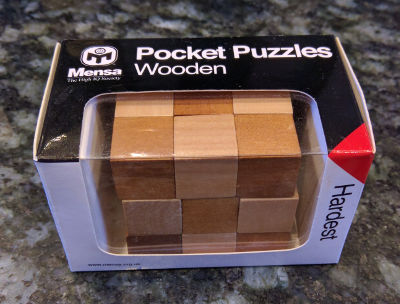
When you take it out the box it looks like this:
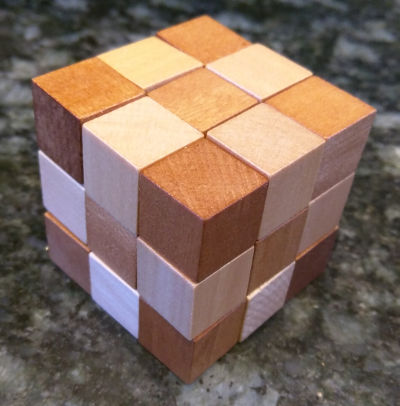
And very soon after it looked like this (which explains why I've christened the puzzle "the snake puzzle"):
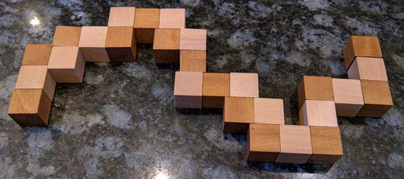
The way it works is that there is a piece of elastic running through each block. On the majority of the blocks the elastic runs straight through, but on some of the it goes through a 90 degree bend. The puzzle is trying to make it back into a cube.
After playing with it a while, I realised that it really is quite hard so I decided to write a program to solve it.
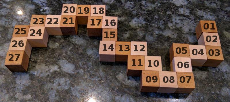
The first thing to do is find a representation for the puzzle. Here is the one I chose:
# definition - number of straight bits, before 90 degree bend
snake = [3,2,2,2,1,1,1,2,2,1,1,2,1,2,1,1,2]
assert sum(snake) == 27
If you look at the picture of it above where it is flattened you can see where the numbers came from. Start from the right hand side.
That also gives us a way of calculating how many combinations there are. At each 90 degree joint, there are 4 possible rotations (ignoring the rotations of the 180 degree blocks) so there are:
4**len(snake)
17 billion combinations. That will include some rotations and reflections, but either way it is a big number.
However it is very easy to know when you've gone wrong with this kind of puzzle - as soon as you place a piece outside of the boundary of the 3x3x3 block you know it is wrong and should try something different.
So how to represent the solution? The way I've chosen is to represent it as a 5x5x5 cube. This is larger than it needs to be but if we fill in the edges then we don't need to do any complicated comparisons to see if a piece is out of bounds. This is a simple trick but it saves a lot of code.
I've also chosen to represent the 3d structure not as a 3d array but as a 1D array (or list in python speak) of length 5 x 5 x 5 = 125.
To move in the x direction you add 1, to move in the y direction you add 5 and to move in the z direction you move 25. This simplifies the logic of the solver considerably - we don't need to deal with vectors.
The basic definitions of the cube look like this:
N = 5
xstride=1    # number of pieces to move in the x direction
ystride=N    # number of pieces to move in the y direction
zstride=N*N  # number of pieces to move in the z direction
In our list we will represent empty space with 0 and space which can't be used with -1:
empty = 0
Now define the empty cube with the boundary round the edges:
# Define cube as 5 x 5 x 5 with filled in edges but empty middle for
# easy edge detection
top = [-1]*N*N
middle = [-1]*5 + [-1,0,0,0,-1]*3 + [-1]*5
cube = top + middle*3 + top
We're going to want a function to turn x, y, z co-ordinates into an index in the cube list:
def pos(x, y, z):
    """Convert x,y,z into position in cube list"""
    return x+y*ystride+z*zstride
So let's see what that cube looks like:
def print_cube(cube, margin=1):
    """Print the cube"""
    for z in range(margin,N-margin):
        for y in range(margin,N-margin):
            for x in range(margin,N-margin):
                v = cube[pos(x,y,z)]
                if v == 0:
                    s = " . "
                else:
                    s = "%02d " % v
                print(s, sep="", end="")
            print()
        print()

print_cube(cube, margin = 0)
-1 -1 -1 -1 -1
-1 -1 -1 -1 -1
-1 -1 -1 -1 -1
-1 -1 -1 -1 -1
-1 -1 -1 -1 -1

-1 -1 -1 -1 -1
-1  .  .  . -1
-1  .  .  . -1
-1  .  .  . -1
-1 -1 -1 -1 -1

-1 -1 -1 -1 -1
-1  .  .  . -1
-1  .  .  . -1
-1  .  .  . -1
-1 -1 -1 -1 -1

-1 -1 -1 -1 -1
-1  .  .  . -1
-1  .  .  . -1
-1  .  .  . -1
-1 -1 -1 -1 -1

-1 -1 -1 -1 -1
-1 -1 -1 -1 -1
-1 -1 -1 -1 -1
-1 -1 -1 -1 -1
-1 -1 -1 -1 -1
Normally we'll print it without the margin.
Now let's work out how to place a segment.
Assuming that the last piece was placed at position we want to place a segment of length in direction. Note the assert to check we aren't placing stuff on top of previous things, or out of the edges:
def place(cube, position, direction, length, piece_number):
    """Place a segment in the cube"""
    for _ in range(length):
        position += direction
        assert cube[position] == empty
        cube[position] = piece_number
        piece_number += 1
    return position
Let's just try placing some segments and see what happens:
cube2 = cube[:] # copy the cube
place(cube2, pos(0,1,1), xstride, 3, 1)
print_cube(cube2)
01 02 03
 .  .  .
 .  .  .

 .  .  .
 .  .  .
 .  .  .

 .  .  .
 .  .  .
 .  .  .
place(cube2, pos(3,1,1), ystride, 2, 4)
print_cube(cube2)
01 02 03
 .  . 04
 .  . 05

 .  .  .
 .  .  .
 .  .  .

 .  .  .
 .  .  .
 .  .  .
place(cube2, pos(3,3,1), zstride, 2, 6)
print_cube(cube2)
01 02 03
 .  . 04
 .  . 05

 .  .  .
 .  .  .
 .  . 06

 .  .  .
 .  .  .
 .  . 07
The next thing we'll need is to undo a place. You'll see why in a moment.
def unplace(cube, position, direction, length):
    """Remove a segment from the cube"""
    for _ in range(length):
        position += direction
        cube[position] = empty
unplace(cube2, pos(3,3,1), zstride, 2)
print_cube(cube2)
01 02 03
 .  . 04
 .  . 05

 .  .  .
 .  .  .
 .  .  .

 .  .  .
 .  .  .
 .  .  .
Now let's write a function which returns whether a move is valid given a current position and a direction and a length of the segment we are trying to place.
def is_valid(cube, position, direction, length):
    """Returns True if a move is valid"""
    for _ in range(length):
        position += direction
        if cube[position] != empty:
            return False
    return True
is_valid(cube2, pos(3,3,1), zstride, 2)
True
is_valid(cube2, pos(3,3,1), zstride, 3)
False
Given is_valid it is now straight forward to work out what moves are possible at a given time, given a cube with a position, a direction and a length we are trying to place.
# directions next piece could go in
directions = [xstride, -xstride, ystride, -ystride, zstride, -zstride]

def moves(cube, position, direction, length):
    """Returns the valid moves for the current position"""
    valid_moves = []
    for new_direction in directions:
        # Can't carry on in same direction, or the reverse of the same direction
        if new_direction == direction or new_direction == -direction:
            continue
        if is_valid(cube, position, new_direction, length):
            valid_moves.append(new_direction)
    return valid_moves
moves(cube2, pos(3,3,1), ystride, 2)
[-1, 25]
So that is telling us that you can insert a segment of length 2 using a direction of -xstride or zstride. If you look at previous print_cube() output you'll see those are the only possible moves.
Now we have all the bits to build a recursive solver.
def solve(cube, position, direction, snake, piece_number):
    """Recursive cube solver"""
    if len(snake) == 0:
        print("Solution")
        print_cube(cube)
        return
    length, snake = snake[0], snake[1:]
    valid_moves = moves(cube, position, direction, length)
    for new_direction in valid_moves:
        new_position = place(cube, position, new_direction, length, piece_number)
        solve(cube, new_position, new_direction, snake, piece_number+length)
        unplace(cube, position, new_direction, length)
This works by being passed in the snake of moves left. If there are no moves left then it must be solved, so we print the solution. Otherwise it takes the head off the snake with length, snake = snake[0], snake[1:] and makes the list of valid moves of that length.
Then we place each move, and try to solve that cube using a recursive call to solve. We unplace the move so we can try again.
This very quickly runs through all the possible solutions:
# Start just off the side
position = pos(0,1,1)
direction = xstride
length = snake[0]
# Place the first segment along one edge - that is the only possible place it can go
position = place(cube, position, direction, length, 1)
# Now solve!
solve(cube, position, direction, snake[1:], length+1)
Solution
01 02 03
20 21 04
07 06 05

16 15 14
19 22 13
08 11 12

17 24 25
18 23 26
09 10 27

Solution
01 02 03
16 15 14
17 24 25

20 21 04
19 22 13
18 23 26

07 06 05
08 11 12
09 10 27
Wow! It came up with 2 solutions! However they are the same solution just rotated and reflected.
But how do you use the solution? Starting from the correct end of the snake, place each piece into its corresponding number. Take the first layer of the solution as being the bottom (or top - whatever is easiest), the next layer is the middle and the one after the top.
After a bit of fiddling around you'll get...
I hope you enjoyed that introduction to puzzle solving with computer.
If you want to try one yourselves, use the same technique to solve solitaire.
IOCCC 2012 Mersenne Prime Checker
2012-10-03 00:00This was my entry for the 20thInternational Obfuscated C Code Contest, a contest whose aims are
- To write the most Obscure/Obfuscated C program under the rules.
- To show the importance of programming style, in an ironic way.
- To stress C compilers with unusual code.
- To illustrate some of the subtleties of the C language.
- To provide a safe forum for poor C code. :-)
I've been meaning to enter the contest for quite a few years so was very pleased to see it re-opened for 2012.
Alas my entry didn't win, but maybe you'll enjoy the entry and explanation.
Here is my entry:
#include<stdio.h>
#include<stdlib.h>
#include<string.h>
#include<inttypes.h>
#define H uint32_t
#define U uint64_t
#define N void
#define T int
#define P calloc(n,sizeof(U))
#define R return
#define I for(
#define M if(
#define E >>32
#define S i=0;i<n;i++)
                      U K=-(U)(H)-1,*B,*C
              ,*x,AC,h;T L,n,F,l,p,D,*_;U e(U x,U
           y){x=K-x;U r=y-x;M y<x)r+=K;R r;}U AB(U x,H
        w,U*c){U s=x+*c;H  t=s<x;*c=(s>>w)+(t<<(64-w));R
     s&((((U)1)<<w)-1             )  ;}  U Q(U x,U y ) {U r
   =x-y;M x<y)r+=K;R r;}                     U AD(U       b,U
  a){H d=b E,c=b;M a >=                      K)a-=           K;a=
  Q(a,c);a=Q(a,d) ;a=e                                         (a
 ,((U)c)<<32);R   a;}U A(                                        U
 x,U y){H a=x,b=  x E,c=y,d
 =y E;x=b*(U)c;y=a*(U)d;U e                                    =a*(
 U)c,f=b*(U)d,t;x+=y;M x<y)f                                   +=1LL
 <<32;t=x<<32;e+=t;M e<t)f+=                                    1;t=
 x E;f+=t;R AD(f,e);}U J(U                                     a,U b
 ){U r= 1;T i;I i=63;i>=0; i--){r=A(r,r);M(b            >>i)&1)r=A(r
  ,a);}R r;}U f(U a){R J(a,K            -2);}N G      (H n,U*x, U*y)
  {T i;I S x[i]=A(x[i],y[i     ]);}N g(   H n,U*x)    {T  i;I S x[i]
=A(x[i],x[i]);}N AA(){U d       = AC;           T k            ;I k=
F;k>=1;k--){T m=1<<k,c=m>>                      1,j,               r
;U w=1;I j=0;j<c;j++){I r=                     0;r<n              ;r
+=m){T a=r+j,b=a+c;U u=x[a]                   ,v=x[b]           ;x[a
]=e(u,v);x[b]=A(Q(u,v),w);}w=                 A(  w,d        );}d=A
(d,d);}}N W(){T k;I k=1;k<=F;k    ++         ){T m=1<<   k,   c=m>>
1,j,r;U z=(U)(1<<((H)F-(H)k)),    d=         J(h,z),w=1;I      j=0
;j<c;j++){I r=0;r<n;r+=m){T a   =r+j,   b=a+ c;U u=x[a], v=A   (w
,x[b]);x[a]=e(u,v);x[b]=Q(u,v);}w=A(w  ,d);}}}T O(){T o=0,i,  w=L
/n;U s=J(7,(K-1)/192/n*5);AC=J(s,192)   ;h=f  (AC   );M 2 *w  +F
>=61)R 0;l=w;D=1<<w;p=w+1;x=P;B=P;C=P;  _= P; *B=1;*C=f(  n);I
i=0;i<=n;i++){U t=(U)L*(U)i,r=t%n,b=t/n ;H               a;M r
E)R 0;M(H)r)b++;M b E)R 0;a=b;M i>0){U c=_[              i-1]
=a-o;M c!=w&&c!=w+1)R 0;M i<n){r=n-r;B[i]=J(s,r);C[i]= f(A(B
[i],n));}}o=a;}R 1;}U V(){T i=0,j=0;U r=0;I;i<64&&j<n;i+=_
[j],j++)r|=x[j]<<i;M r)R r;I r=j=0;j<n;j++)r|=x[j];R r;}
N X(H c,T i){while(c){I;i<n;i++){H y=1<<_[i];x[i]+=c;
M x[i]>=y)x[             i]-=y,c=1;            else
R;}i=0;}                     }N Y(H     c){T    i;
while(c)   {I S{H y=1<<        _[i]     ;x[i    ]-=
c;M x[i]>=y)x[i]+=y,c=1        ;else    R     ;}}}N
Z(U c){T i;while(c){I          S{x[    i]=AB(x[i],_[i],
&c);H t=c;M!(c E)&&t         <D){M t ) X(t,i+1);R;}}}}N q()
{T i;U c=0;G(n,x,         B);AA(F,x);g(n,x);W(F       ,x);G(n,x
,C);I S x[i]=          AB(x[i],_[i],&c);M c)Z(c);Y    (2);}T main(
T w,char**         v){T i,k,j;M w<2)       {puts("Usage: p [n]");R 1
;}L=atoi                       (v[1]       );j=w>2    ?atoi(v[2]):L-
2;do F++                       ,n=1<<F;while(!O          ());I k=0;k
<1;k++){*x=4;I i=0;i<j;i++)q();}printf("0x%016"PRIX64"\n",V());R 0;}
I'm going to explain exactly what it does and how, but first here are the hints and remarks I provided with the code. Some of the hints assume you've pre-processed the code into something vaguely legible first.
Hints
You stare at the source code... Is that a picture of a monk? What does that strange mathematical writing say? You get a subliminal message... Hunt for primes? But how?
You run the program. It comes up with a strange usage message. What could "p" be? You try running the program with a prime number as an argument.
./prog 23209
It returns after a few seconds with the rather cryptic message
0x0000000000000000
What could that mean? Maybe that 223209-1 (a 6,987 digit number) is prime after all?
OK If you haven't guessed by now, this program proves the primality of Mersenne primes of the form 2p-1. The biggest known primes are of this form because there is an efficient test for primality - the Lucas Lehmer test.
If you run the program and it produces 0x0000000000000000 (0 in hex) as an answer then you've found a prime of the form 2p-1. If it produces anything else then 2p-1 isn't prime. The printed result is the bottom 64 bits of the last iteration of the Lucas Lehmer test.
Have a look at the source code and see if you can work out how it implements the Lucas Lehmer test...
Your first clue is to work out what the magic number -(U)(H)-1 is. (My favourite bit of obfuscation!)
Got it? It is a prime just less than 264, 0xFFFFFFFF00000001 = 264 - 232 + 1 (p from now on), with some rather special properties.
The most important of which is that arithmetic modulo p can all be done without using divisions or modulo operations (which are really slow). See if you can spot the add, subtract and multiplication routines. There are also reciprocal and to the power operations in there somewhere.
The next important property is that p-1 has the following factors
2^32 * 3 * 5 * 17 * 257 * 65537
All those factors of 2 suggest that we can do a Fast Fourier Transform over the Galois Field GF(p) which is arithmetic modulo p. See if you can spot the FFT code!
To make a truly efficient Mersenne primality prover it is necessary to implement the IBDWT a variant of the FFT using an irrational base. This halves the size of the FFT array by combining the modulo and multiply steps from the Lucas Lehmer test into one. You might wonder how you can use an irrational base in a discrete field where every element is an integer, but as it happens the p chosen has n-th roots of 2 where n is up to 26, which means that an IBDWT can be defined for FFT sizes up to 226.
You'll find the code to generate the roots of 1 and 2 necessary for the IBDWT if you search for 7 in the code. 7 is a primitive root of GF(p) so all follows from that!
This all integer IBDWT isn't susceptible to the round off errors that plague the floating point implementation, but does suffer in the speed stakes from the fact that modern CPUs have much faster floating point units than integer units.
For example to check if 218000000-1 is prime (a 5,418,539 digit number) Prime95 (the current speed demon) uses a 220 FFT size and each iteration takes it about 25ms. On similar hardware it this program takes about 1.2s also using an FFT size of 220! Prime95 is written in optimised assembler to use SSE3 whereas this program was squeezed into 2k of portable C with a completely unoptimised FFT!
This program can do an FFT of up to 226 entries. Each entry can have up to 18 bits in (as 2*18+26 <= 63), which means that the biggest exponent that it can test for primality is 18*226-1 = 1,207,959,551. This would be number of 363 million decimal digits so could be used to find a 100 million digit prime and scoop the EFF $150,000 prize! It would take rather a long time though...
The second argument to the program allows the number of iterations to be put in, and using this it has been validated against the Prime95 test suite. There is a unit test for the program but I thought including it was probably against the spirit of the contest!
Speed of the FFT could be improved greatly, but unfortunately there wasn't space in the margin to do so ;-)
Remarks about the Code
This should compile on any compiler which supports inttypes.h from the C99 standard (eg gcc).
It runs a lot quicker when compiled as a 64 bit binary!
I have successfully compiled and run this program without changes or compiler warnings for:
- 64 bit Ubuntu Linux 11.10
- 32 bit Debian Linux (Lenny)
- Windows using MINGW
- OS X 10.7 using Apple's gcc based compiler
If you don't have a compiler which supports inttypes.h from C99 (hello it is 2012 Microsoft!) then you'll need to go platform specific:
- comment out the #include <inttypes.h> line
- change the #define for uint32_t to be an unsigned 32 bit type unsigned int or unsigned __int32
- change the #define for uint64_t to be an unsigned 64 bit type unsigned long long or unsigned __int64
- add #define PRIX64 "llX" or "lX" or "I64X"
How it was written
I wrote most of this code some time ago as a view to publishing a full description of how my ARMprime code works in easy to understand C rather than a twisty turny mess of ARM assembler macros.
However I never got round to finishing it, so I used the IOCCC as a spur to get me to finish it properly!
I've open-sourced the code and the build chain at github.
As you can imagine it isn't possible to develop the code in the form above from scratch! I created an unobfuscated version mersenne.c first and then wrote two programs, one which compresses the code (it uses a manual version of LZ77 compression with #define statements) and another which makes it into the pretty picture.
This means that I can change the code and just type make to create the final pretty code for the entry, and to run the unit tests with.
The first challenge was cutting the code down to size. It needed to be less than 2k of non-whitespace characters and less than 4k total. I went through it getting rid of all extraneous functions, compacting definitions, removing optimisations, obfuscating and it was still far too big.
With the help of crush.py and after many hours of work I managed to get it small enough. I then wrote check.py to see whether the code was within the competition rules and unit_test.py to validate the code against Prime95's test suite.
Finally I wrote artify.py which reads the crushed source code and uses it to paint the image. It treats each character (or sometimes a group of characters so the C remains valid) as a pixel and paints the image with code!
Note that none of the python programs are particularly tidy, but that python is a really good language for doing this in - I'd hate to be doing it in C!
How it works
Now I've introduced the unobfuscated version, I can show how each part of the code works.
Firstly all good obfuscated programs have lots of global variables to shorten the code down:
u64 MOD_P =  -(u64)(u32)-1,         /* 0xFFFFFFFF00000001 - the magic number */
    *digit_weight,                  /* Array of weights for IBDWT */
    *digit_unweight,                /* Inverse of the above */
    *x,                             /* pointer to array of n 64 bit integers - the current number */
    MOD_W,                          /* The root of 2 for the fft so that 2**MOD_W == 1 mod p */
    MOD_INVW;                       /* The inverse of the above so that MOD_W * MOD_INVW == 1 mod p */

int exponent,                       /* The mersenne exponent - we are testing 2^exponent -1 is prime or not */
    n,                              /* The number of 64 bit numbers in the FFT */
    log_n,                          /* n = 2^log_n */
    digit_width0,                   /* Digit width for the IBDWT */
    digit_width1,
    digit_width_0_max,
    *digit_widths;                  /* Array of number of bits in each element of the FFT */
From the top down there is the main loop which contains the Lucas Lehmer algorithm:
int main(int w, char ** v)
{
    int i,k,j;
    if (w < 2)
    {
        puts("Usage:@p@[n]");
        return 1;
    }

    exponent = atoi(v[1]);
    j = w > 2 ? atoi(v[2]) : exponent - 2; /* iterations */
    /* initialise, finding correct FFT size */
    do log_n++, n = 1 << log_n;
    while(!mersenne_initialise());

    for (k = 0; k < 1; k++)
    {
        *x = 4;
        for (i = 0; i < j; i++)
            mersenne_mul();
    }
    printf("0x%016" PRIX64 "\n", mersenne_residue());
    return 0;
}
It reads the exponent and optional number of iterations from the command line, then initialises the program, starting with a small FFT size n and increasing until it finds one which fits.
It then does the Lucas Lehmer test setting the initial value to 4, iterating it for exponent times and printing the residue.
The core of the Lucas Lehmer test (and the IBDWT) is the mersenne_mul function which squares the current number and subtracts 2, returning it modulo 2p - 1
void mersenne_mul()
{
    int i;
    u64 c = 0;

    /* weight the input */
    mod_vector_mul(n, x, digit_weight);

    /* transform */
    fft_fastish(log_n, x);

    /* point multiply */
    mod_sqr_vector(n, x);

    /* untransform */
    invFft_fastish(log_n, x);

    /* unweight and normalise the output */
    mod_vector_mul(n, x, digit_unweight);

    /* carry propagation */
    for (i = 0; i < n; i++)
        x[i] = mod_adc(x[i], digit_widths[i], &c);
    if (c)
        mersenne_add64(c);

    /* subtract 2 */
    mersenne_sub32(2);
}
This the FFT, point multiply and inverse FFT perform a convolution. This does the bulk of the work of the multiplication. The weight and unweight and the start and end is the IBDWT which ensures that the result is modulo 2 p - 1. The carries are propagated and 2 is subtracted from the end.
The FFT is a completely standard FFT with bit reversed output, the only unusual thing being that all the operations are mod p rather than with complex numbers. If you compare the code for the FFT with a standard implementation you will see it is very similar:
void fft_fastish()
{
    u64 d = MOD_W;
    int k;

    for (k = log_n; k >= 1; k--)
    {
        int m = 1 << k,
            c = m >> 1,
            j,
            r;
        u64 w = 1;
        for (j = 0; j < c; j++)
        {
            for (r = 0; r < n; r += m)
            {
                int a = r + j,
                    b = a + c;
                u64 u = x[a],
                    v = x[b];
                x[a] = mod_add(u, v);
                x[b] = mod_mul(mod_sub(u, v), w);
            }
            w = mod_mul(w, d);
        }
        d = mod_mul(d, d);
    }
}
MOD_W is the root of unity the FFT is built on. It happens to be an integer in GF(p) such that MOD_Wn == 1 mod p. You can see the FFT calculating the twiddles (w). Precalculating them would be better obviously but not in 2k of code! The inner loop shows the butterfly.
Now for the fundamental operations over GF(p). First thing to note is that in the code p = MOD_P = 264 - 232 + 1. MOD_P was chosen so that it has quite a few special properties, one of them being that it is possible to do modulo p operations without doing divisions (which are really slow!).
The easiest operation to define is subtraction:
u64 mod_sub(u64 x, u64 y)
{
    u64 r = x - y;
    /* if borrow generated - hopefully the compiler will optimise this! */
    if (x < y)
        r += MOD_P;        /* Add back p if borrow */
    return r;
}
The C code was designed so that the if statement should be optimised into a jump on carry flag if the compiler is doing its job properly. Addition can then be defined as subtracting a negative number:
u64 mod_add(u64 x, u64 y)
{
    x = MOD_P - x;        /* do addition by negating y then subtracting */
    u64 r = y - x;        /* y - (-x) */
    /* if borrow generated - hopefully the compiler will optimise this! */
    if (y < x)
        r += MOD_P;        /* Add back p if borrow */
    return r;
}
To do multiplication, first it is necessary to work out how to do reduce a 128 bit number mod p. We use these facts:
Thus to reduce a 128 bit number mod p (split into 32 bit chunks x3,x2,x1,x0):
This is explained in more detail in my ARMprime pages. This division free code then looks like this:
u64 mod_reduce(u64 b, u64 a)
{
    u32 d = b >>32,
        c = b;
    if (a >= MOD_P)                /* (x1, x0) */
        a -= MOD_P;
    a = mod_sub(a, c);
    a = mod_sub(a, d);
    a = mod_add(a, ((u64)c)<<32);
    return a;
}
Given mod_reduce, multiplication is relatively straight forward:
u64 mod_mul(u64 x, u64 y)
{
    u32 a = x,
        b = x >>32,
        c = y,
        d = y >>32;

    /* first synthesise the product using 32*32 -> 64 bit multiplies */
    x = b * (u64)c;
    y = a * (u64)d;
    u64 e = a * (u64)c,
        f = b * (u64)d,
        t;

    x += y;                        /* b*c + a*d */
    /* carry? */
    if (x < y)
        f += 1LL << 32;            /* carry into upper 32 bits - can't overflow */

    t = x << 32;
    e += t;                        /* a*c + LSW(b*c + a*d) */
    /* carry? */
    if (e < t)
        f += 1;                    /* carry into upper 64 bits - can't overflow*/
    t = x >>32;
    f += t;                        /* b*d + MSW(b*c + a*d) */
    /* can't overflow */

    /* now reduce: (b*d + MSW(b*c + a*d), a*c + LSW(b*c + a*d)) */
    return mod_reduce(f, e);
}
The definitions for the other arithmetic operations are straight forward now. Power is just repeated multiplication and squaring. Inverse is to the power of -1.
All those things come together in the mersenne_mul function above!
If you want to look at the complete (mostly) unobfuscated code then take look through mersenne.c.
Conclusion
The IOCCC was a fun challenge and it got me to finally complete my C conversion of a lot of really difficult ARM assembly code. Hopefully I'll find the time to demonstrate some more optimised FFTs and an FFT with a factor of 3 in too.
Getting the code small enough was really, really difficult, but helped immensely by Python. It started off life as pretty obscure so that process made it more so! I'm afraid even as explained above it probably isn't accessible to very many people - my apologies for that.
Happy Prime Hunting!
How I Solved the GCHQ challenge
2011-12-04 20:00This is an unsanitised account of how I solved the GCHQ challenge at http://www.canyoucrackit.co.uk/. According to the BBC the competition began in secret on the 3rd of November 2011 and will continue until the 12th of December. I was going to hold back this publication until the contest ended but a solution has just made it to the front page of slashdot so I think the jig is up!
This writeup includes the wrong turnings I took and the bad assumptions I made along the way so any reader can see the kind of thought processes necessary. I very deliberately did no searching on the Internet about the puzzle so all the work below (and the mistakes) are mine alone!
The programs linked to in the article are the final versions, I didn't keep the intermediate versions which I talk about in the text, so you'll have to imagine what they looked like.
Warning
This article contains spoilers on how to do the challenge - don't read any further if you want to solve it yourself!
Stage 1
The challenge opens showing a single image with a load of hex digits in and a form to submit your answer. The image looks like this:
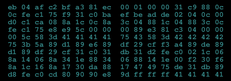
The first thing I did was to decode the hex data. Using a python program of course! I played around with trying to get it to display an image. It is obviously low entropy but what is it? Not an image anyway.
I used cyber.py to save it to a binary file and ran the unix "file" utility on it which told me it was x86 code:
$ file cyber.bin
cyber.bin: DOS executable (COM)
Interesting. A disassembly was required cyber.disassembly.asm:
x86dis -r 0 160 -s intel < cyber.bin > cyber.disassembly.asm
The code appeared to be linux flavour, exiting politely with the correct int 0x80 call.
The obvious next step is to run the code. It is bare code which you can't just run on any modern OS. I could have added headers to it but I decided to write cyber.c to load it into memory instead. I used mmap to map a padded version of the code so I could get the code and the stack under my control and examine it after the code had exited:
gcc -g -m32 -Wall -static -o cyber cyber.c
Running the code, it seemed to be early terminating - needing 0x42424242 or "BBBB" on the end to continue according to this bit of code:
0000004A 58                                 pop     eax
0000004B 3D 42 42 42 42                     cmp     eax, 0x42424242
00000050 75 3B                              jnz     0x0000008D ; exit
I tried padding with "BBBB" and it core dumped this time. After studying the disassembly some more and experimenting I noted that it needed "BBBB" and a 4 byte length. Running that it appears to decrypt something on the stack this time, so I'm getting somewhere.
But what to decrypt? I needed a string starting with "BBBB". I recursively downloaded the entire website and grepped it for "BBBB" without success. However on really close examination of a hex dump of cyber.png I discovered this:
00000050: 1233 7e39 c170 0000 005d 6954 5874 436f  .3~9.p...]iTXtCo
00000060: 6d6d 656e 7400 0000 0000 516b 4a43 516a  mment.....QkJCQj
00000070: 4941 4141 4352 3250 4674 6343 4136 7132  IAAACR2PFtcCA6q2
00000080: 6561 4338 5352 2b38 646d 442f 7a4e 7a4c  eaC8SR+8dmD/zNzL
00000090: 5143 2b74 6433 7446 5134 7178 384f 3434  QC+td3tFQ4qx8O44
000000a0: 3754 4465 755a 7735 502b 3053 7362 4563  7TDeuZw5P+0SsbEc
000000b0: 5952 0a37 386a 4b4c 773d 3d32 cabe f100  YR.78jKLw==2....
That string "QkJCQj...78jKLw==" with upper and lower case letters, '+' and '/' and the trailing '==' screams base64 encoding to me. I decoded it in python and it decodes to BBBB2\x00\x00\x00\x91... - hooray a string starting with "BBBB" and a sensible looking length! I then modified cyber.py to add that on the end of the code and ran the cyber.c binary. After it had ran I examined the stack in the cyber.bin.padded file originally written by cyber.py. I saw this:
00002c0: 00 00 00 00 00 00 00 00 00 00 47 45 54 20 2f 31  ..........GET /1
00002d0: 35 62 34 33 36 64 65 31 66 39 31 30 37 66 33 37  5b436de1f9107f37
00002e0: 37 38 61 61 64 35 32 35 65 35 64 30 62 32 30 2e  78aad525e5d0b20.
00002f0: 6a 73 20 48 54 54 50 2f de e6 fb 2f ef ae 5d aa  js HTTP/.../..].
Which looks very like an HTTP transaction, ie a coded instruction to fetch a file, so I did:
$ wget http://www.canyoucrackit.co.uk/15b436de1f9107f3778aad525e5d0b20.js
Stage 2
The downloaded file 15b436de1f9107f3778aad525e5d0b20.js is a description of a VM with an initial state, but no code to implement the VM. It has a very realistic and amusing initial commment! It also says "stage 2 of 3" which is the first indication how long this challenge is going to be.
Otherwise it seems a reasonably straightforward job to implement the VM and I got cracking on vm.py after reading that. Note that it has 8 bytes of 'firmware' which don't seem to fit in anywhere which is a bit puzzling.
Wasted a lot of time trying to get the VM to work. Tried poking the firmware in various imaginitive places. Found a few bugs then finally re-read the doc again - Ah-ha it is 16 byte segment size, not a 16 bit register... Duh!
Fixed that and it runs much better now actually decrypting stuff and halts properly.
Found this in the memory in final.core after vm.py had run:
00001c0: 47 45 54 20 2f 64 61 37 35 33 37 30 66 65 31 35  GET /da75370fe15
00001d0: 63 34 31 34 38 62 64 34 63 65 65 63 38 36 31 66  c4148bd4ceec861f
00001e0: 62 64 61 61 35 2e 65 78 65 20 48 54 54 50 2f 31  bdaa5.exe HTTP/1
00001f0: 2e 30 00 00 00 00 00 00 00 00 00 00 00 00 00 00  .0..............
That seems like an instruction to fetch something from the web site again:
$ wget http://www.canyoucrackit.co.uk/da75370fe15c4148bd4ceec861fbdaa5.exe
Haven't used the firmware - wonder where that fits in...
Stage 3
I looked in da75370fe15c4148bd4ceec861fbdaa5.exe - and found it to be a windows x86 executable. It seems to be using the cygcrypt dll from cygwin and the crypt() function. It has a string in it which looks exactly like a DES password crypt "hqDTK7b8K2rvw". I then set John the Ripper and crack off on it for good measure to find the encrypted password.
John the Ripper found the password cyberwin in 2 hours. The easy one was my test to make sure it was working:
Loaded 2 password hashes with 2 different salts (Traditional DES [128/128 BS SSE2-16])
easy             (trivial)
cyberwin         (test)
guesses: 2  time: 0:02:01:42 (3)  c/s: 1537K  trying: cufqnm5! - cyberwen
Use the "--show" option to display all of the cracked passwords reliably
And double checking with python:
>>> crypt("cyberwin", "hq") == "hqDTK7b8K2rvw"
True
Meanwhile I tried running the exe on windows but it doesn't run without that dll.
After installing cygwin with the "crypt" package which has the correct dll in, I copied cygcrypt-0.dll and cygwin1.dll into my working directory. The exe now runs and gives:
>da75370fe15c4148bd4ceec861fbdaa5.exe

keygen.exe

usage: keygen.exe hostname

>da75370fe15c4148bd4ceec861fbdaa5.exe localhost

keygen.exe

error: license.txt not found
I then tried it with "cyberwin" in license.txt:
>da75370fe15c4148bd4ceec861fbdaa5.exe localhost

keygen.exe

error: license.txt invalid
Hmm, I was expecting that to work.
Looking through the keygen.edit.asm (my annotated version) I discovered that the password should be prefixed with "gchq". The first hint as to who set this puzzle!
cmp    [ebp+var_38], 71686367h ; gchq
jnz    short invalid_license
Putting "gchqcyberwin" into the license.txt and running the program goes better this time. It fetches a page this time, but it is a 404 not found. Note that this isn't the normal 404 page because the exe uses HTTP/1.0 rather than HTTP/1.1:
>da75370fe15c4148bd4ceec861fbdaa5.exe www.canyoucrackit.co.uk

keygen.exe

loading stage1 license key(s)...
loading stage2 license key(s)...

request:

GET /hqDTK7b8K2rvw/0/0/0/key.txt HTTP/1.0

response:

HTTP/1.1 404 Not Found
Content-Type: text/html; charset=us-ascii
Server: Microsoft-HTTPAPI/2.0
Date: Sat, 03 Dec 2011 09:29:29 GMT
Connection: close
Content-Length: 315

<!DOCTYPE HTML PUBLIC "-//W3C//DTD HTML 4.01//EN""http://www.w3.org/TR/html4/strict.dtd">
<HTML><HEAD><TITLE>Not Found</TITLE>
<META HTTP-EQUIV="Content-Type" Content="text/html; charset=us-ascii"></HEAD>
<BODY><h2>Not Found</h2>
<hr><p>HTTP Error 404. The requested resource is not found.</p>
</BODY></HTML>
Trying the above in the web browser gives the normal 404 message. Trying with telnet see that it needs HTTP/1.0. HTTP/1.1 with host header gives normal page. Trying "GET / HTTP/1.0" gives the same message so probably a red herring to do with the server (or not see later!).
The fact that the page isn't found means that there is something missing. But what? The code is executing the equivalent of this to make the GET string to fetch the page:
sprintf(buffer, "GET /%s/%x/%x/%x/key.txt HTTP/1.0\r\n\r\n", crypted_string, key1, key2, key2);
However key1, key2 and key3 are all 0 which doesn't look right. I tried some things for those missing %x parameters:
>>> t = "gchqcyberwin"
>>> from struct import *
>>> [ "%x" %x  for x in unpack(">iii", t) ]
['67636871', '63796265', '7277696e']
>>> [ "%x" %x  for x in unpack("<iii", t) ]
['71686367', '65627963', '6e697772']
wget http://www.canyoucrackit.co.uk/hqDTK7b8K2rvw/71686367/65627963/6e697772/key.txt
wget http://www.canyoucrackit.co.uk/hqDTK7b8K2rvw/67636871/63796265/7277696e/key.txt
But no luck.
More study of the keygen.edit.asm disassembly reveals that key1, key2, key3 come from the end of the license.txt file after "gchqcyberwin". So that makes 24 bytes of secrets read from the licence file which is the size of the buffer the code allocates.
Ah-Ha! The clue is in the "loading stageX license key(s)..." messages.
This bit of assembler code gives it away (annotations by me):
loc_4011A5:             ; "loading stage1 license key(s)...\n"
mov     [esp+78h+var_78], offset aLoadingStage1L
call    printf
mov     eax, [ebp+var_2C]       ; copy 4 bytes of the licence file
mov     [ebp+var_48], eax
mov     [esp+78h+var_78], offset aLoadingStage2L ; "loading stage2 license key(s)...\n\n"
call    printf
mov     eax, [ebp+var_28]       ; ...and another 4 bytes
mov     [ebp+var_44], eax
mov     eax, [ebp+var_24]       ; ..and another 4 bytes
mov     [ebp+var_40], eax
It prints "loading stage1 license keys(s)..." loads 4 bytes, then "loading stage2 license key(s)..." and loads 8 bytes. Stage 1 is the first stage of the puzzle - need 4 bytes from this - how about the unused 4 bytes at the start of the code that is jumped over "af c2 bf a3". Stage2 is the second stage from which we need 8 bytes - the mysteriously unused firmware seems appropriate.
I wrote keyfetch.py to fiddle with the endianess and after a bit of trial and error it worked:
GET 'http://www.canyoucrackit.co.uk/hqDTK7b8K2rvw/a3bfc2af/d2ab1f05/da13f110/key.txt'
Pr0t3ct!on
Fetched using HTTP/1.1 and the GET program. Which looks like it could be the password! But it doesn't work :-(
The headers showed nothing interesting. I then tried using keygen.exe with a corrected license file - it didn't work as I expected as the webserver doesn't support HTTP/1.0 (or maybe I did something wrong).
However trying it by hand using telnet and HTTP/1.0 does do something different:
$ telnet www.canyoucrackit.co.uk 80
Trying 31.222.164.161...
Connected to www.canyoucrackit.co.uk.
Escape character is '^]'.
GET http://www.canyoucrackit.co.uk/hqDTK7b8K2rvw/a3bfc2af/d2ab1f05/da13f110/key.txt HTTP/1.0

HTTP/1.1 200 OK
Content-Type: text/plain
Last-Modified: Wed, 26 Oct 2011 08:40:14 GMT
Accept-Ranges: bytes
ETag: "bc46bae1ba93cc1:0"
Server: Microsoft-IIS/7.5
Date: Sun, 04 Dec 2011 11:14:54 GMT
Connection: close
Content-Length: 37

Pr0t3ct!on#cyber_security@12*12.2011+Connection closed by foreign host.
$
I reworked keyfetch.py to make the fetch using HTTP/1.0 to double check.
Trying Pr0t3ct!on#cyber_security@12*12.2011+ as the key does indeed work and produces this page: http://www.canyoucrackit.co.uk/soyoudidit.asp:
So you did it. Well done! Now this is where it gets interesting. Could you use your skills and ingenuity to combat terrorism and cyber threats? As one of our experts, you'll help protect our nation's security and the lives of thousands. Every day will bring new challenges, new solutions to find – and new ways to prove that you're one of the best.
I'm not going to apply for a job as I'm rather fully employed elsewhere, but it was a fun challenge!
Postmortem
I didn't see this until the 1st December 2011 when a colleague at work (thanks Tom!) mentioned it to me and I didn't have time to work on it until Friday the 2nd of December. It took me one very late night on Friday and intermittent hacking on Saturday and Sunday to complete the challenge - about 12 hours in total. I spent 3 hours tracking down that mis-understanding in vm.py about 16 byte segments and 2 hours trying to work out what the missing 12 bytes were in the URL in stage 3.
I think Stage 1 was very hard - perhaps deliberately so. Stage 2 was much easier - there was a defined goal and any competent computer scientist would be able to knock up the VM code. Stage 3 involved an awful lot of reading C compiler created x86 assembler which was painful. I suspect I could have done it a lot quicker if I'd had some better tools. An interactive disassembling debugger would have been useful - I used to have such a thing when I did 68000 programming and it was a wonder.
I note that I didn't actually have to crack the encrypted password in Stage 3. I could have just changed one byte and have it ignore the check but I was expecting that the code would actually need to use it. Alas no and so much for John the Ripper!
Finally thanks to GCHQ for making the challenge - it was a good one!
Pi - Chudnovsky
2011-10-08 00:00In Part 3 we managed to calculate 1,000,000 decimal places of π with Machin's arctan formula. Our stated aim was 100,000,000 places which we are going to achieve now!
We have still got a long way to go though, and we'll have to improve both our algorithm (formula) for π and our implementation.
The current darling of the π world is the Chudnovsky algorithm which is similar to the arctan formula but it converges much quicker. It is also rather complicated. The formula itself is derived from one by Ramanjuan who's work was extraordinary in the extreme. It isn't trivial to prove, so I won't! Here is Chudnovsky's formula for π as it is usually stated:
![\[ \frac{1}{\pi} = 12 \sum^\infty_{k=0} \frac{(-1)^k (6k)! (13591409 + 545140134k)}{(3k)!(k!)^3 640320^{3k + 3/2}} \]](https://www.craig-wood.com/nick/images/math/13e67da9779a237b0d3b4b0fa5d70d12.png)
That is quite a complicated formula, we will make more comprehensible in a moment. If you haven't seen the Σ notation before it just like a sum over a for loop in python. For example:
![\[ \sum^{10}_{k=1} k^2 \]](https://www.craig-wood.com/nick/images/math/b63b93c8cb0658657d92a47f208b2a99.png)
Is exactly the same as this python fragment:
sum(k**2 for k in range(1,11))
First let's get rid of that funny fractional power:

Now let's split it into two independent parts. See how there is a + sign inside the Σ? We can split it into two series which we will call a and b and work out what π is in terms of a and b:

Finally note that we can calculate the next a term from the previous one, and the b terms from the a terms which simplifies the calculations rather a lot.

OK that was a lot of maths! But it is now in an easy to compute state, which we can do like this:
def pi_chudnovsky(one=1000000):
    """
    Calculate pi using Chudnovsky's series

    This calculates it in fixed point, using the value for one passed in
    """
    k = 1
    a_k = one
    a_sum = one
    b_sum = 0
    C = 640320
    C3_OVER_24 = C**3 // 24
    while 1:
        a_k *= -(6*k-5)*(2*k-1)*(6*k-1)
        a_k //= k*k*k*C3_OVER_24
        a_sum += a_k
        b_sum += k * a_k
        k += 1
        if a_k == 0:
            break
    total = 13591409*a_sum + 545140134*b_sum
    pi = (426880*sqrt(10005*one, one)*one) // total
    return pi
We need to be able to take the square root of long integers which python doesn't have a built in for. Luckily this is easy to provide. This uses a square root algorithm devised by Newton which doubles the number of significant places in the answer (quadratic convergence) each iteration:
 def sqrt(n, one):
     """
     Return the square root of n as a fixed point number with the one
     passed in.  It uses a second order Newton-Raphson convergence.  This
     doubles the number of significant figures on each iteration.
     """
     # Use floating point arithmetic to make an initial guess
     floating_point_precision = 10**16
     n_float = float((n * floating_point_precision) // one) / floating_point_precision
     x = (int(floating_point_precision * math.sqrt(n_float)) * one) // floating_point_precision
     n_one = n * one
     while 1:
         x_old = x
         x = (x + n_one // x) // 2
         if x == x_old:
             break
     return x
It uses normal floating point arithmetic to make an initial guess then refines it using Newton's method.
See pi_chudnovsky.py for the complete program. When I run it I get this:
Digits Time (seconds) 10 4.696e-05 100 0.0001530 1000 0.002027 10000 0.08685 100000 8.453 1000000 956.3Which is nearly 3 times quicker than the best result in part 3, and gets us 1,000,000 places of π in about 15 minutes.
Amazingly there are still two major improvements we can make to this. The first is to recast the calculation using something called binary splitting. Binary splitting is a general purpose technique for speeding up this sort of calculation. What it does is convert the sum of the individual fractions into one giant fraction. This means that you only do one divide at the end of the calculation which speeds things up greatly, because division is slow compared to multiplication.
Consider the general infinite series
![\[ S(0,\infty) = \frac{a_0p_0}{b_0q_0} + \frac{a_1p_0p_1}{b_1q_0q_1} + \frac{a_2p_0p_1p_2}{b_2q_0q_1q_2} + \frac{a_3p_0p_1p_2p_3}{b_3q_0q_1q_2q_3} + \cdots \]](https://www.craig-wood.com/nick/images/math/b1178e265167bde29ef15a32724b03ea.png)
This could be used as a model for all the infinite series we've looked at so far. Now lets consider the partial sum of that series from terms a to b (including a, not including b).

This is a part of the infinite series, and if a=0 and b=∞ it becomes the infinite series above.
Now lets define some extra functions:

Let's define m which is a <= m <= b. Making m as near to the middle of a and b will lead to the quickest calculations, but for the proof, it has to be somewhere between them. Lets work out what happens to our variables P, Q, R and T when we split the series in two:

The first three of those statements are obvious from the definitions, but the last deserves proof.
![\begin{eqnarray*} \lefteqn{B(m,b)Q(m,b)T(a,m) + B(a,m)P(a,m)T(m,b) = } \\ & & \left[T(a,b) = B(a,b)Q(a,b)S(a,b)\right] \\ &=& B(m,b)Q(m,b)B(a,m)Q(a,m)S(a,m) + B(a,m)P(a,m)B(m,b)Q(m,b)S(m,b) \\ & & \left[Q(a,b) = Q(a,m)Q(b,m)\right] \\ & & \left[B(a,b) = B(a,m)B(b,m)\right] \\ &=& B(a,b)Q(a,b)S(a,m) + B(a,b)P(a,m)Q(m,b)S(m,b) \\ &=& B(a,b)(Q(a,b)S(a,m) + P(a,m)Q(m,b)S(m,b)) \\ & & \left[Q(m,b) = \frac{Q(a,b)}{Q(a,m)}\right] \\ &=& B(a,b)\left(Q(a,b)S(a,m) + \frac{Q(a,b)P(a,m)}{Q(a,m)}S(m,b)\right) \\ &=& B(a,b)Q(a,b)\left(S(a,m) + \frac{P(a,m)}{Q(a,m)}S(m,b)\right) \\ &=& B(a,b)Q(a,b)\left( \frac{a_ap_a}{b_aq_a} + \frac{a_{a+1}p_ap_{a+1}}{b_{a+1}q_aq_{a+1}} + \frac{a_{a+2}p_ap_{a+1}p_{a+2}}{b_{a+2}q_aq_{a+1}q_{a+2}} + \cdots + \frac{a_{m-1}p_ap_{a+1}p_{a+2}\cdots p_{m-1}}{b_{m-1}q_aq_{a+1}\cdots p_{m-1}} + \frac{p_ap_{a+1}\cdots p_{m-1}}{q_aq_{a+1}\cdots q_{m-1}} + \left(\frac{a_mp_m}{b_mq_m} + \frac{a_{m+1}p_mp_{m+1}}{b_{m+1}q_mq_{m+1}} + \frac{a_{m+2}p_mp_{m+1}p_{m+2}}{b_{m+2}q_mq_{m+1}q_{m+2}} + \cdots + \frac{a_{b-1}p_mp_{m+1}p_{m+2}\cdots p_{b-1}}{b_{b-1}q_mq_{m+1}\cdots p_{b-1}} \right)\right) \\ &=& B(a,b)Q(a,b)\left( \frac{a_ap_a}{b_aq_a} + \frac{a_{a+1}p_ap_{a+1}}{b_{a+1}q_aq_{a+1}} + \frac{a_{a+2}p_ap_{a+1}p_{a+2}}{b_{a+2}q_aq_{a+1}q_{a+2}} + \cdots + \frac{a_{m-1}p_ap_{a+1}p_{a+2}\cdots p_{m-1}}{b_{m-1}q_aq_{a+1}\cdots p_{m-1}} + \frac{p_ap_{a+1}\cdots p_{m-1}}{q_aq_{a+1}\cdots q_{m-1}} + \frac{a_mp_ap_{a+1}\cdots p_m}{b_mq_aq_{a+1}\cdots q_m} + \frac{a_{m+1}p_ap_{a+1}\cdots p_{m+1}}{b_{m+1}q_aq_{a+1}\cdots q_{m+1}} + \frac{a_{m+2}p_ap_{a+1}\cdots p_{m+2}}{b_{m+2}q_aq_{a+1}\cdots q_{m+2}} + \cdots + \frac{a_{b-1}p_ap_{a+1}\cdots p_{b-1}}{b_{b-1}q_aq_{a+1}\cdots p_{b-1}} \right) \\ &=& B(a,b)Q(a,b)S(a,b) \\ &=& T(a,b) \\ \end{eqnarray*}](https://www.craig-wood.com/nick/images/math/2ba1a65b212b89c3bd3b1f83350a5827.png)
We can use these relations to expand the series recursively, so if we want S(0,8) then we can work out S(0,4) and S(4,8) and combine them. Likewise to calculate S(0,4) and S(4,8) we work out S(0,2), S(2,4), S(4,6), S(6,8) and combine them, and to work out those we work out S(0,1), S(1,2), S(2,3), S(3,4), S(4,5), S(5,6), S(6,7), S(7,8). Luckily we don't have to split them down any more as we know what P(a,a+1), Q(a,a+1) etc is from the definition above.

And when you've finally worked out P(0,n),Q(0,n),B(0,n),T(0,n) you can work out S(0,n) with

If you want a more detailed and precise treatment of binary splitting then see Bruno Haible and Thomas Papanikolaou's paper.
So back to Chudnovksy's series. We can now set these parameters in the above general formula:

This then makes our Chudnovksy pi function look like this:
def pi_chudnovsky_bs(digits):
    """
    Compute int(pi * 10**digits)

    This is done using Chudnovsky's series with binary splitting
    """
    C = 640320
    C3_OVER_24 = C**3 // 24
    def bs(a, b):
        """
        Computes the terms for binary splitting the Chudnovsky infinite series

        a(a) = +/- (13591409 + 545140134*a)
        p(a) = (6*a-5)*(2*a-1)*(6*a-1)
        b(a) = 1
        q(a) = a*a*a*C3_OVER_24

        returns P(a,b), Q(a,b) and T(a,b)
        """
        if b - a == 1:
            # Directly compute P(a,a+1), Q(a,a+1) and T(a,a+1)
            if a == 0:
                Pab = Qab = 1
            else:
                Pab = (6*a-5)*(2*a-1)*(6*a-1)
                Qab = a*a*a*C3_OVER_24
            Tab = Pab * (13591409 + 545140134*a) # a(a) * p(a)
            if a & 1:
                Tab = -Tab
        else:
            # Recursively compute P(a,b), Q(a,b) and T(a,b)
            # m is the midpoint of a and b
            m = (a + b) // 2
            # Recursively calculate P(a,m), Q(a,m) and T(a,m)
            Pam, Qam, Tam = bs(a, m)
            # Recursively calculate P(m,b), Q(m,b) and T(m,b)
            Pmb, Qmb, Tmb = bs(m, b)
            # Now combine
            Pab = Pam * Pmb
            Qab = Qam * Qmb
            Tab = Qmb * Tam + Pam * Tmb
        return Pab, Qab, Tab
    # how many terms to compute
    DIGITS_PER_TERM = math.log10(C3_OVER_24/6/2/6)
    N = int(digits/DIGITS_PER_TERM + 1)
    # Calclate P(0,N) and Q(0,N)
    P, Q, T = bs(0, N)
    one = 10**digits
    sqrtC = sqrt(10005*one, one)
    return (Q*426880*sqrtC) // T
Hopefully you'll see how the maths above relates to this as I've used the same notation in each. Note that we calculate the number of digits of pi we expect per term of the series (about 14.18) to work out how many terms of the series we need to compute, as the binary splitting algorithm needs to know in advance how many terms to calculate. We also don't bother calculating B(a) as it is always 1. Defining a function inside a function like this makes what is known as a closure. This means that the inner function can access the variables in the outer function which is very convenient in this recursive algorithm as it stops us having to pass the constants to every call of the function.
See pi_chudnovsky_bs.py for the complete program. When I run it I get this:
Digits Time (seconds) 10 1.096e-05 100 3.194e-05 1000 0.0004899 10000 0.03403 100000 3.625 1000000 419.1This is a bit more than twice as fast as pi_chudnovsky.py giving us our 1,000,000 places in just under 7 minutes. If you profile it you'll discover that almost all the time spent in the square root calculations (86% of the time) whereas only 56 seconds is spent in the binary splitting part. We could spend time improving the square root algorithm, but it is time to bring out the big guns: gmpy.
Gmpy is a python interface to the gmp library which is a C library for arbitrary precision arithmetic. It is very fast, much faster than the built in int type in python for large numbers. Luckily gmpy provides a type (mpz) which works exactly like normal python int types, so we have to make hardly any changes to our code to use it. These are using initialising variables with the mpz type, and using the sqrt method on mpz rather than our own home made sqrt algorithm:
import math
from gmpy2 import mpz
from time import time

def pi_chudnovsky_bs(digits):
    """
    Compute int(pi * 10**digits)

    This is done using Chudnovsky's series with binary splitting
    """
    C = 640320
    C3_OVER_24 = C**3 // 24
    def bs(a, b):
        """
        Computes the terms for binary splitting the Chudnovsky infinite series

        a(a) = +/- (13591409 + 545140134*a)
        p(a) = (6*a-5)*(2*a-1)*(6*a-1)
        b(a) = 1
        q(a) = a*a*a*C3_OVER_24

        returns P(a,b), Q(a,b) and T(a,b)
        """
        if b - a == 1:
            # Directly compute P(a,a+1), Q(a,a+1) and T(a,a+1)
            if a == 0:
                Pab = Qab = mpz(1)
            else:
                Pab = mpz((6*a-5)*(2*a-1)*(6*a-1))
                Qab = mpz(a*a*a*C3_OVER_24)
            Tab = Pab * (13591409 + 545140134*a) # a(a) * p(a)
            if a & 1:
                Tab = -Tab
        else:
            # Recursively compute P(a,b), Q(a,b) and T(a,b)
            # m is the midpoint of a and b
            m = (a + b) // 2
            # Recursively calculate P(a,m), Q(a,m) and T(a,m)
            Pam, Qam, Tam = bs(a, m)
            # Recursively calculate P(m,b), Q(m,b) and T(m,b)
            Pmb, Qmb, Tmb = bs(m, b)
            # Now combine
            Pab = Pam * Pmb
            Qab = Qam * Qmb
            Tab = Qmb * Tam + Pam * Tmb
        return Pab, Qab, Tab
    # how many terms to compute
    DIGITS_PER_TERM = math.log10(C3_OVER_24/6/2/6)
    N = int(digits/DIGITS_PER_TERM + 1)
    # Calclate P(0,N) and Q(0,N)
    P, Q, T = bs(0, N)
    one_squared = mpz(10)**(2*digits)
    sqrtC = (10005*one_squared).sqrt()
    return (Q*426880*sqrtC) // T
See pi_chudnovsky_bs_gmpy.py for the complete program. When I run it I get this:
Digits Time (seconds) 10 1.597e-05 100 3.409e-05 1000 0.003403 10000 0.003571 100000 0.09120 1000000 1.760 10000000 30.11 100000000 542.2So we have achieved our goal of calculating 100,000,000 places of π in just under 10 minutes! What is limiting the program now is memory... 100,000,000 places takes about 600MB of memory to run. With 6 GB of free memory it could probably calculate one billion places in a few hours.
What if we wanted to go faster? Well you could use gmp-chudnovsky.c which is a C program which implements the Chudnovsky Algorithm. It is heavily optimised and rather difficult to understand, but if you untangle it you'll see it does exactly the same as above, with one extra twist. The twist is that it factors the fraction in the binary splitting phase as it goes along. If you examine the gmp-chudnovsky.c results page you'll see that the little python program above acquits itself very well - the python program only takes 75% longer than the optimised C program on the same hardware.
One algorithm which has the potential to beat Chudnovsky is the Arithmetic Geometric Mean algorithm which doubles the number of decimal places each iteration. It involves square roots and full precision divisions which makes it tricky to implement well. In theory it should be faster than Chudnovsk but, so far, in practice Chudnovsky is faster.
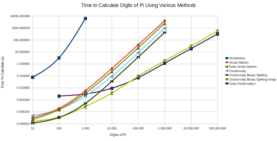
Here is a chart of all the different π programs we've developed in Part 1, Part 2, Part 3 and Part 4 with their timings on my 2010 Intel® Core™ i7 CPU Q820 @ 1.73GHz running 64 bit Linux:
Pi - Machin
2011-07-19 00:00In Part 2 we managed to calculate 100 decimal places of π with Archimedes' recurrence relation for π which was a fine result, but we can do bigger and faster.
To go faster we'll have to use a two pronged approach - a better algorithm for π, and a better implementation.
In 1706 John Machin came up with the first really fast method of calculating π and used it to calculate π to 100 decimal places. Quite an achievement considering he did that entirely with pencil and paper. Machin's formula is:
π/4 = 4cot⁻¹(5) - cot⁻¹(239)
    = 4tan⁻¹(1/5) - tan⁻¹(1/239)
    = 4 * arctan(1/5) - arctan(1/239)
We can prove Machin's formula using some relatively easy math! Hopefully you learnt this trigonometric formula at school:
![\[ tan(a + b) = \frac{tan(a) + tan(b)}{1 - tan(a) \cdot tan(b)} \]](https://www.craig-wood.com/nick/images/math/ba59c45582fef5d43cb00b4239b38ea4.png)
Substitute a = arctan(x) and b = arctan(y) into it, giving:
![\[ tan(arctan(x) + arctan(y)) = \frac{tan(arctan(x)) + tan(arctan(y)}{1 - tan(arctan(x)) \cdot tan(arctan(y))} \]](https://www.craig-wood.com/nick/images/math/fe543c13b0d71c92c76a4d793965744b.png)
Note that tan(arctan(x)) = x which gives:
![\[ tan(arctan(x) + arctan(y)) = \frac{x + y}{1 - xy} \]](https://www.craig-wood.com/nick/images/math/141c9b63ef2ce9bc7b029f6e7f19121c.png)
arctan both sides to get:
![\[ arctan(x) + arctan(y) = arctan\left(\frac{x + y}{1 - xy}\right) \]](https://www.craig-wood.com/nick/images/math/35c7a3b474febc099202d94d8d6884af.png)
This gives us a method for adding two arctans. Using this we can prove Machin's formula with a bit of help from python's fractions module:
>>> from fractions import Fraction
>>> def add_arctan(x, y): return (x + y) / (1 - x * y)
...
>>> a = add_arctan(Fraction(1,5), Fraction(1,5))
>>> a # 2*arctan(1/5)
Fraction(5, 12)
>>> b = add_arctan(a, a)
>>> b # 4*arctan(1/5)
Fraction(120, 119)
>>> c = add_arctan(b, Fraction(-1,239))
>>> c # 4*arctan(1/5) - arctan(1/239)
Fraction(1, 1)
>>>
So Machin's formula is equal to arctan(1/1) = π/4 QED! Or if you prefer it written out in mathematical notation:

So how do we use Machin's formula to calculate π? Well first we need to calculate arctan(x) which sounds complicated, but we've seen the infinite series for it already in Part 1 :
![\[ arctan(x) = x - \frac{x^3}{3} + \frac{x^5}{5} - \frac{x^7}{7} + \frac{x^9}{9} - \cdots ( -1 <= x <= 1 ) \]](https://www.craig-wood.com/nick/images/math/f4ec0d0c341574593cce1f5f41c5737a.png)
We can see that if x=1/5 then the terms get smaller very quickly, which means that the series will converge quickly. Let's substitute x = 1/x and get:
![\[ arctan(1/x) = \frac{1}{x} - \frac{1}{3x^3} + \frac{1}{5x^5} - \frac{1}{7x^7} + \frac{1}{9x^9} - \cdots ( x >= 1 ) \]](https://www.craig-wood.com/nick/images/math/1a80bfa0baaf1b2171d10afda4973766.png)
Each term in the series is created by dividing the previous term by a small integer. Dividing two 100 digit numbers is hard work as I'm sure you can imagine from your experiences with long division at school! However it is much easier to divide a short number (a single digit) into a 100 digit number. We called this short division at school, and that is the key to making a much faster π algorithm. In fact if you are dividing an N digit number by an M digit number it takes rougly N*M operations. That square root we did in Part 2 did dozens of divisions of 200 digit numbers. So if we could somehow represent the current term in a int [1] then we could use this speedy division to greatly speed up the calculation.
The way we do that is to multiply everything by a large number, lets say 10 100. We then do all our calculations with integers, knowing that we should shift the decimal place 100 places to the left when done to get the answer. This needs a little bit of care, but is a well known technique known as fixed point arithmetic.
The definition of the arctan(1/x) function then looks like this:
def arctan(x, one=1000000):
    """
    Calculate arctan(1/x)

    arctan(1/x) = 1/x - 1/3*x**3 + 1/5*x**5 - ... (x >= 1)

    This calculates it in fixed point, using the value for one passed in
    """
    power = one // x            # the +/- 1/x**n part of the term
    total = power               # the total so far
    x_squared = x * x           # precalculate x**2
    divisor = 1                 # the 1,3,5,7 part of the divisor
    while 1:
        power = - power // x_squared
        divisor += 2
        delta = power // divisor
        if delta == 0:
            break
        total += delta
    return total
The value one passed in is the multiplication factor as described above. You can think of it as representing 1 in the fixed point arithmetic world. Note the use of the // operator which does integer divisions. If you don't use this then python will make floating point values [2]. In the loop there are two divisions, power // x_squared and power // divisor. Both of these will be dividing by small numbers, x_squared will be 5² = 25 or 239² = 57121 and divisor will be 2 * the number of iterations which again will be small.
So how does this work in practice? On my machine it calculates 100 digits of π in 0.18 ms which is over 30,000 times faster than the previous calculation with the decimal module in Part 2!
Can we do better?
Well the answer is yes! Firstly there are better arctan formulae. Amazingly there are other formulae which will calculate π too, like these, which are named after their inventors:
def pi_machin(one):
    return 4*(4*arctan(5, one) - arctan(239, one))

def pi_ferguson(one):
    return 4*(3*arctan(4, one) + arctan(20, one) + arctan(1985, one))

def pi_hutton(one):
    return 4*(2*arctan(3, one) + arctan(7, one))

def pi_gauss(one):
    return 4*(12*arctan(18, one) + 8*arctan(57, one) - 5*arctan(239, one))
It turns out that Machin's formula is really very good, but Gauss's formula is slightly better.
The other way we can do better is to use a better formula for arctan(). Euler came up with this accelerated formula for arctan:
![\[ arctan(1/x) = \frac{x}{1+x^2} + \frac{2}{3}\frac{x}{(1+x^2)^2} + \frac{2\cdot4}{3\cdot5}\frac{x}{(1+x^2)^3} + \frac{2\cdot4\cdot6}{3\cdot5\cdot7}\frac{x}{(1+x^2)^4} + \cdots \]](https://www.craig-wood.com/nick/images/math/180899b6c341c96a41270221b9c97621.png)
This converges to arctan(1/x) at the roughly the same rate per term than the formula above, however each term is made directly from the previous term by multiplying by 2n and dividing by (2n+1)(1+x²). This means that it can be implemented with only one (instead of two) divisions per term, and hence runs roughly twice as quickly. If we implement this in python in fixed point, then it looks like this:
def arctan_euler(x, one=1000000):
    """
    Calculate arctan(1/x) using euler's accelerated formula

    This calculates it in fixed point, using the value for one passed in
    """
    x_squared = x * x
    x_squared_plus_1 = x_squared + 1
    term = (x * one) // x_squared_plus_1
    total = term
    two_n = 2
    while 1:
        divisor = (two_n+1) * x_squared_plus_1
        term *= two_n
        term = term // divisor
        if term == 0:
            break
        total += term
        two_n += 2
    return total
Notice how we pre-calculate as many things as possible (like x_squared_plus_1) to get them out of the loop.
See the complete program: pi_artcan_integer.py. Here are some timings [3] of how the Machin and the Gauss arctan formula fared, with and without the accelerated arctan.
Formula Digits Normal Arctan (seconds) Euler Arctan (seconds) Machin 10 3.004e-05 2.098e-05 Gauss 10 2.098e-05 1.907e-05 Machin 100 0.0001869 0.0001471 Gauss 100 0.0001869 0.0001468 Machin 1000 0.005599 0.003520 Gauss 1000 0.005398 0.003445 Machin 10000 0.3995 0.2252 Gauss 10000 0.3908 0.2186 Machin 100000 38.33 21.69 Gauss 100000 37.44 21.12 Machin 1000000 3954.1 2396.8 Gauss 1000000 3879.4 2402.1There are several interesting things to note. Firstly that we just calculated 1,000,000 decimal places of π in 40 minutes! Secondly that to calculate 10 times as many digits it takes 100 times as long. This means that our algorithm scales as O(n²) where n is the number of digits. So if 1,000,000 digits takes an hour, 10,000,000 would take 100 hours (4 days) and 100,000,000 would take 400 days (13 months). Your computer might run out of memory, or explode in some other fashion when calculating 100,000,000 digits, but doesn't seem impossible any more.
The Gauss formula is slightly faster than the Machin for nearly all the results. The accelerated arctan formula is 1.6 times faster than the normal arctan formula so that is a definite win.
A billion (1,000,000,000) digits of pi would take about 76 years to calculate using this program which is a bit out of our reach! There are several ways we could improve this. If we could find an algorithm for calculating π which was quicker than O(n²), or if we could find an O(n²) algorithm which just ran a lot faster. We could also throw more CPUs at the problem. To see how this might be done, we could calculate all the odd terms on one processor, and all the even terms on another processor for the arctan formula and add them together at the end.. That would run just about twice as quickly. That could easily be generalised to lots of processors:
arctan(1/x) = 1/x - 1/3x³ + 1/5x⁵ - 1/7x⁷ + ...
            = 1/x         + 1/5x⁵ -       + ... # run on cpu 1
            +     - 1/3x³         - 1/7x⁷ + ... # run on cpu 2
So if we had 76 CPU cores, we could probably calculate π to 1,000,000,000 places in about a year.
There are better algorithms for calculating π though, and there are faster ways of doing arithmetic than python's built in long integers. We'll explore both in Part 4!
[1]Python's integer type was called called long in python 2, just int in python 3[2]Unless you are using python 2[3]All timings generated on my 2010 Intel® Core™ i7 CPU Q820 @ 1.73GHz running 64 bit LinuxRecommend
About Joyk
Aggregate valuable and interesting links.
Joyk means Joy of geeK