Smooth Voxel Terrain (Part 2)

Last time we formulated the problem of isosurface extraction and discussed some general approaches at a high level. Today, we’re going to get very specific and look at meshing in particular.

For the sake of concreteness, let us suppose that we have approximated our potential field $f$ by sampling it onto a cubical grid at some fixed resolution. To get intermediate values, we’ll just interpolate between grid points using the standard trilinear interpolation. This is like a $C^0$ generalization of Minecraft-style voxel surfaces. Our goal in this article is to figure out how to extract a mesh of the implicit surface (or zero-crossings of $f$ ). In particular, we’re going to look at three different approaches to this problem:

Marching Cubes

By far the most famous method for extracting isosurfaces is the marching cubes algorithm. In fact, it is so popular that the term `marching cubes’ is even more popular than the term `isosurface’ (at least according to Google)! It’s quite a feat when an algorithm becomes more popular than the problem which it solves! The history behind this method is very interesting. It was originally published back in SIGGRAPH 87, and then summarily patented by the Lorensen and Cline. This fact has caused a lot of outrage, and is been widely cited as one of the classic examples of patents hampering innovation. Fortunately, the patent on marching cubes expired back in 2005 and so today you can freely use this algorithm in the US with no fear of litigation.

Much of the popularity of marching cubes today is due in no small part to a famous article written by Paul Bourke. Back in 1994 he made a webpage called “Polygonizing a Scalar Field”, which presented a short, self-contained reference implementation of marching cubes (derived from some earlier work by Cory Gene Bloyd.) That tiny snippet of a C program is possibly the most copy-pasted code of all time. I have seen some variation of Bloyd/Bourke’s code in every implementation of marching cubes that I’ve ever looked at, without exception. There are at least a couple of reasons for this:

Paul Bourke’s exposition is really good. Even today, with many articles and tutorials written on the technique, none of them seem to explain it quite as well. (And I don’t have any delusions that I will do any better!)
Also their implementation is very small and fast. It uses some clever tricks like a precalculated edge table to speed up vertex generation. It is difficult to think of any non-trivial way to improve upon it.
Finally, marching cubes is incredibly difficult to code from scratch.

This last point needs some explaining, Conceptually, marching cubes is rather simple. What it does is sample the implicit function along a grid, and then checks the sign of the potential function at each point (either +/-). Then, for every edge of the cube with a sign change, it finds the point where this edge intersects the volume and adds a vertex (this is just like ray casting a bunch of tiny little segments between each pair of grid points). The hard part is figuring out how to stitch some surface between these intersection points. Up to the position of the zero crossings, there are $2^8 = 256$ different possibilities, each of which is determined by the sign of the function at the 8 vertices of the cube:

Some of the marching cubes special cases. (c) Wikipedia, created by Jean-Marie Favreau.

Even worse, some of these cases are ambiguous! The only way to resolve this is to somewhat arbitrarily break the symmetry of the table based on a case-by-case analysis. What a mess! Fortunately, if you just download Bloyd/Bourke’s code, then you don’t have to worry about any of this and everything will just work. No wonder it gets used so much!

Marching Tetrahedra

Both the importance of isosurface extraction and the perceived shortcomings of marching cubes motivated the search for alternatives. One of the most popular was the marching tetrahedra, introduced by Doi and Koide. Besides the historical advantage that marching tetrahedra was not patented, it does have a few technical benefits:

Marching tetrahedra does not have ambiguous topology, unlike marching cubes. As a result, surfaces produced by marching tetrahedra are always manifold.
The amount of geometry generated per tetrahedra is much smaller, which might make it more suitable for use in say a geometry shader.
Finally, marching tetrahedra has only $2^4 = 16$ cases, a number which can be further reduced to just 3 special cases by symmetry considerations. This is enough that you can work them out by hand.

Exercise: Try working out the cases for marching tetrahedra yourself. (It is really not bad.)

The general idea behind marching tetrahedra is the same as marching cubes, only it uses a tetrahedral subdivision. Again, the standard reference for practical implementation is Paul Bourke (same page as before, just scroll down a bit.) While there is a lot to like about marching tetrahedra, it does have some draw backs. In particular, the meshes you get from marching tetrahedra are typically about 4x larger than marching cubes. This makes both the algorithm and rendering about 4x slower. If your main consideration is performance, you may be better off using a cubical method. On the other hand, if you really need a manifold mesh, then marching tetrahedra could be a good option. The other nice thing is that if you are obstinate and like to code everything yourself, then marching tetrahedra may be easier since there aren’t too many cases to check.

The Primal/Dual Classification

By now, both marching cubes and tetrahedra are quite old. However, research into isosurface extraction hardly stopped in the 1980s. In the intervening years, many new techniques have been developed. One general class of methods which has proven very effective are the so-called `dual’ schemes. The first dual method, surface nets, was proposed by Sarah Frisken Gibson in 1999:

S.F. Gibson, (1999) “Constrained Elastic Surface Nets” Mitsubishi Electric Research Labs, Technical Report.

The main distinction between dual and primal methods (like marching cubes) is the way they generate surface topology. In both algorithms, we start with the same input: a volumetric mesh determined by our samples, which I shall take the liberty of calling a sample complex for lack of a better term. If you’ve never heard of the word cell complex before, you can think of it as an n-dimensional generalization of a triangular mesh, where the `cells’ or facets don’t have to be simplices.

In the sample complex, vertices (or 0-cells) correspond to the sample points; edges (1-cells) correspond to pairs of nearby samples; faces (2-cells) bound edges and so on:

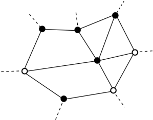
Here is an illustration of such a complex. I’ve drawn the vertices where the potential function is negative black, and the ones where it is positive white.

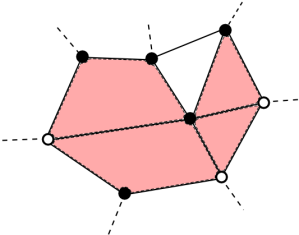
Both primal and dual methods walk over the sample complex, looking for those cells which cross the 0-level of the potential function. In the above illustration, this would include the following faces:

Primal Methods

Primal methods, like marching cubes, try to turn the cells crossing the bounary into an isosurface using the following recipe:

Edges crossing the boundary become vertices in the isosurface mesh.
Faces crossing the boundary become edges in the isosurface mesh.
n-cells crossing the boundary become (n-1)-cells in the isosurface mesh.

One way to construct a primal mesh for our sample complex would be the following:

This is pretty nice because it is easy to find intersection points along edges. Of course, there is some topological ambiguity in this construction. For non-simplicial cells crossing the boundary it is not always clear how you would glue the cells together:

primalcell.png?w=300&h=63

As we have seen, these ambiguities lead to exponentially many special cases, and are generally a huge pain to deal with.

Dual Methods

Dual methods on the other hand use a very different topology for the surface mesh. Like primal methods, they only consider the cells which intersect the boundary, but the rule they use to construct surface cells is very different:

For every edge crossing the boundary, create an (n-1) cell. (Face in 3D)
For every face crossing the boundary, create an (n-2) cell. (Edge in 3D)
For every d-dimensional cell, create an (n-d) cell.
For every n-cell, create a vertex.

This creates a much simpler topological structure:

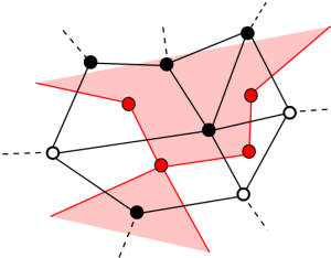
The nice thing about this construction is that unlike primal methods, the topology of the dual isosurface mesh is completely determined by the sample complex (so there are no ambiguities). The disadvantage is that you may sometimes get non-manifold vertices:

dualmesh.png?w=300&h=124

Make Your Own Dual Scheme

To create your own dual method, you just have to specify two things:

A sample complex.
And a rule to assign vertices to every n-cell intersecting the boundary.

The second item is the tricky part, and much of the research into dual methods has focused on exploring the possibilities. It is interesting to note that this is the opposite of primal methods, where finding vertices was pretty easy, but gluing them together consistently turned out to be quite hard.

Surface Nets

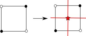
Here’s a neat puzzle: what happens if we apply the dual recipe to a regular, cubical grid (like we did in marching cubes)? Well, it turns out that you get the same boxy, cubical meshes that you’d make in a Minecraft game (topologically speaking)!

Left: A dual mesh with vertex positions snapped to integer coordinates. Right: A dual mesh with smoothed vertex positions.

So if you know how to generate Minecraft meshes, then you already know how to make smooth shapes! All you have to do is squish your vertices down onto the isosurface somehow. How cool is that?

This technique is called “surface nets” (remember when we mentioned them before?) Of course the trick is to figure out where you place the vertices. In Gibson’s original paper, she formulated the process of vertex placement as a type of global energy minimization and applied it to arbitrary smooth functions. Starting with some initial guess for the point on the surface (usually just the center of the box), her idea is to perturb it (using gradient descent) until it eventually hits the surface somewhere. She also adds a spring energy term to keep the surface nice and globally smooth. While this idea sounds pretty good in theory, in practice it can be a bit slow, and getting the balance between the energy terms just right is not always so easy.

Naive Surface Nets

Of course we can often do much better if we make a few assumptions about our functions. Remember how I said at the beginning that we were going to suppose that we approximated $f$ by trilinear filtering? Well, we can exploit this fact to derive an optimal placement of the vertex in each cell — without having to do any iterative root finding! In fact, if we expand out the definition of a trilinear filtered function, then we can see that the 0-set is always a hyperboloid. This suggests that if we are looking for a 0-crossings, then a good candidate would be to just pick the vertex of the hyperboloid.

Unfortunately, calculating this can be a bit of a pain, so let’s do something even simpler: Rather than finding the optimal vertex, let’s just compute the edge crossings (like we did in marching cubes) and then take their center of mass as the vertex for each cube. Surprisingly, this works pretty well, and the mesh you get from this process looks similar to marching cubes, only with fewer vertices and faces. Here is a side-by-side comparison:

Left: Marching cubes. Right: Naive surface nets.

Another advantage of this method is that it is really easy to code (just like the naive/culling algorithm for generating Minecraft meshes.) I’ve not seen this technique published or mentioned before (probably because it is too trivial), but I have no doubt someone else has already thought of it. Perhaps one of you readers knows a citation or some place where it is being used in practice? Anyway, feel free to steal this idea or use it in your own projects. I’ve also got a javascript implementation that you can take a look at.

Dual Contouring

Say you aren’t happy with a mesh that is bevelled. Maybe you want sharp features in your surface, or maybe you just want some more rigorous way to place vertices. Well my friend, then you should take a look at dual contouring:

T. Ju, F. Losasso, S. Schaefer, and J. Warren. (2004) “Dual Contouring of Hermite Data” SIGGRAPH 2004

Dual contouring is a very clever solution to the problem of where to place vertices within a dual mesh. However, it makes a very big assumption. In order to use dual contouring you need to know not only the value of the potential function but also its gradient! That is, for each edge you must compute the point of intersection AND a normal direction. But if you know this much, then it is possible to reformulate the problem of finding a nice vertex as a type of linear least squares problem. This technique produces very high quality meshes that can preserve sharp features. As far as I know, it is still one of the best methods for generating high quality meshes from potential fields.

Of course there are some downsides. The first problem is that you need to have Hermite data, and recovering this from an arbitrary function requires using either numerical differentiation or applying some clunky automatic differentiator. These tools are nice in theory, but can be difficult to use in practice (especially for things like noise functions or interpolated data). The second issue is that solving an overdetermined linear least squares problem is much more expensive than taking a few floating point reciprocals, and is also more prone to blowing up unexpectedly when you run out of precision. There is some discussion in the paper about how to manage these issues, but it can become very tricky. As a result, I did not get around to implementng this method in javascript (maybe later, once I find a good linear least squares solver…)

As usual, I made a WebGL widget to try all this stuff out (caution: this one is a bit browser heavy):

Click here to try the demo in your browser!

This tool box lets you compare marching cubes/tetrahedra and the (naive) surface nets that I described above. The Perlin noise examples use the javascript code written by Kas Thomas. Both the marching cubes and marching tetrahedra algorithms are direct ports of Bloyd/Bourke’s C implementation. Here are some side-by-side comparisons.

Left-to-right: Marching Cubes (MC), Marching Tetrahedra (MT), Surface Nets (SN)

MC: 15268 verts, 7638 faces. MT: 58580 verts, 17671 faces. SN: 3816 verts, 3701 faces.

MC: 1140 verts, 572 faces. MT: 4200 verts, 1272 faces. SN: 272 verts, 270 faces.

MC: 80520 verts, 40276 faces. MT: 302744 verts, 91676 faces. SN: 20122 verts, 20130 faces.

MC: 172705 verts, 88071 faces. MT: 639522 verts, 192966 faces. SN: 41888 verts, 40995 faces.

A few general notes:

The controls are left mouse to rotate, right mouse to pan, and middle mouse to zoom. I have no idea how this works on Macs.
I decided to try something different this time and put a little timing widget so you can see how long each algorithm takes. Of course you really need to be skeptical of those numbers, since it is running in the browser and timings can fluctuate quite randomly depending on totally arbitrary outside forces. However, it does help you get something of a feel for the relative performance of each method.
In the marching tetrahedra example there are frequently many black triangles. I’m not sure if this is because there is a bug in my port, or if it is a problem in three.js. It seems like the issue might be related to the fact that my implementation mixes quads and triangles in the mesh, and that three.js does not handle this situation very well.
I also didn’t implement dual contouring. It isn’t that much different than surface nets, but in order to make it work you need to get Hermite data and solve some linear least squares problems, which is hard to do in Javascript due to lack of tools.

Benchmarks

To compare the relative performance of each method, I adapted the experimental protocol described in my previous post. As before, I tested the experiments on a sample sinusoid, varying the frequency over time. That is, I generated a volume $65^3$ volume plot of

$\sin( \frac{n \pi}{2} x ) + \sin( \frac{n \pi}{2} y ) + \sin( \frac{n \pi}{2} z )$

Over the range $[ - \frac{\pi}{2}, + \frac{\pi}{2} ]^3$ . Here are the timings I got, measured in milliseconds

Frequency Marching Cubes Marching Tetrahedra Surface Nets 0 29.93 57 24.06 1 43.62 171 29.42 2 61.48 250 37.78 3 93.31 392 47.72 4 138.2 510 51.36 5 145.8 620 74.54 6 186 784 83.99 7 213.2 922 97.34 8 255.9 1070 112.4 9 272.1 1220 109.2 10 274.6 1420 124.3

By far marching tetrahedra is the slowest method, mostly on account of it generating an order of magnitude more triangles. Marching cubes on the other hand, despite generating nearly 2x as many primitives was still pretty quick. For small geometries both marching cubes and surface nets perform comparably. However, as the isosurfaces become more complicated, eventually surface nets win just on account of creating fewer primitives. Of course this is a bit like comparing apples-to-oranges, since marching cubes generates triangles while surface nets generate quads, but even so surface nets still produce slightly less than half as many facets on the benchmark. To see how they stack up, here is a side-by-side comparison of the number of primitives each method generates for the benchmark:

Frequency Marching Cubes Marching Tetrahedra Surface Nets 0 0 0 0 1 15520 42701 7569 2 30512 65071 14513 3 46548 102805 22695 4 61204 130840 29132 5 77504 167781 37749 6 92224 197603 43861 7 108484 233265 52755 8 122576 263474 58304 9 139440 298725 67665 10 154168 329083 73133

Conclusion

Each of the isosurface extraction methods has their relative strengths and weaknesses. Marching cubes is nice on account of the free and easily usable implementations, and it is also pretty fast. (Not to mention it is also the most widely known.) Marching tetrahedra solves some issues with marching cubes at the expense of being much slower and creating far larger meshes. On the other hand surface nets are much faster and can be extended to generate high quality meshes using more sophisticated vertex selection algorithms. It is also easy to implement and produces slightly smaller meshes. The only downside is that it can create non-manifold vertices, which may be a problem for some applications. I unfortunately never got around to properly implementing dual contouring, mostly because I’d like to avoid having to write a robust linear least squares solver in javascript. If any of you readers wants to take up the challenge, I’d be interested to see what results you get.

I’ve been messing around with the wordpress theme a lot lately. For whatever reason, it seems like the old one I was using would continually crash Chrome. I’ve been trying to find something nice and minimalist. Hopefully this one works out ok.

Smooth Voxel Terrain (Part 2)