

Bayesian Machine Learning: MCMC, Latent Dirichlet Allocation and Probabilistic P...
source link: https://sandipan-dey.medium.com/mcmc-and-probabilistic-programming-17bf43c7c9fc
Go to the source link to view the article. You can view the picture content, updated content and better typesetting reading experience. If the link is broken, please click the button below to view the snapshot at that time.
Bayesian Machine Learning: MCMC, Latent Dirichlet Allocation and Probabilistic Programming with Python
Implementing the Random-Walk Metropolis-Hastings and Gibbs Sampling Algorithms to Approximate the Posterior Distribution + Topic Modeling with Latent Dirichlet Allocation with Collapsed Gibbs Sampling + Probabilistic Programming using PyMC3
In this blog we shall focus on sampling and approximate inference by Markov chain Monte Carlo (MCMC). This class of methods can be used to obtain samples from a probability distribution, e.g. a posterior distribution. The samples aproximately represent the distribution, and can be used to approximate expectations. The problems we shall work on appeared in an assignment here. Next, we shall learn how to use a library for probabilistic programming and inference called PyMC3. These problems appeared in an assignment in the coursera course Bayesian Methods for Machine Learning by UCSanDiego HSE. Some of the problems statements are taken from the course.

The Metropolis-Hastings algorithm is useful for approximate computation of the posterior distribution, since the exact computation of posterior distribution is often infeasible, the partition function being computationally intractable.
The following figure describes how to sample from a distribution known upto a (normalizing) constant, using the Metropolis-Hastings algorithm.

Let’s first define a function mh() implementing the Metropolis Hasting algorithm, using the Gaussian proposal distribution above. The function should take as arguments
and return [θ(1) , . . . , θ(S) ] — a list of S samples from p(θ) ∝ p∗(θ).
import numpy as npfrom scipy.stats import multivariate_normaldef mh(p_star, param_init, num_samples=5000, stepsize=1.0): theta = param_init samples = np.zeros((num_samples+1, param_init.shape[0])) samples[0] = theta for i in range(num_samples): theta_cand = multivariate_normal(mean=theta, \ cov=[stepsize**2]*len(theta))\ .rvs(size=1) a = min(1, p_star(theta_cand)/p_star(theta)) u = np.random.uniform() if u < a: theta = theta_cand samples[i+1] = theta return samples
Let’s use the following function to plot the samples generated.
def plot_samples(samples, p_star=multivariate_normal(mean=np.zeros(2), cov=np.identity(2)).pdf): plt.figure(figsize=(10,5)) X, Y = np.meshgrid(np.linspace(-3,3,100), np.linspace(-3,3,100)) Z = p_star(np.stack([X, Y], axis=-1)) plt.subplot(121), plt.grid() plt.contourf(X, Y, Z) plt.subplot(122), plt.grid() plt.scatter(samples[:,0], samples[:,1], alpha=0.25) plt.show()
samples = mh(p_star=multivariate_normal(mean=np.zeros(2)).pdf, \ param_init=np.zeros(2))plot_samples(samples)

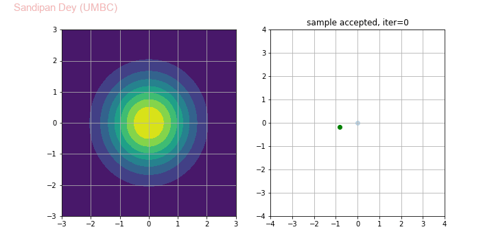
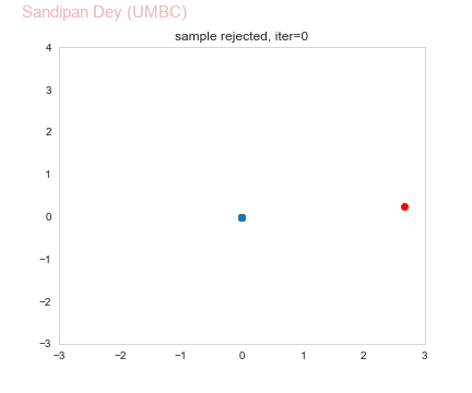
The following animation shows how the Metropolis-Hasting Algorithm works for stepsize=1. The left subplot shows the contours of the original bivariate Gaussian. On the right subplot, the green samples correspond to the ones accepted and red ones correspond to the ones rejected.
- Let’s sample another 5,000 points from p(x, y)=N(x; 0, 1)N(y; 0, 1) using the function mh() with ε=1, but this time initialize at x=7, y=7.
- Let’s generate a scatter plot of the drawn samples and notice the first 20 samples.
- As expected, the plot probably shows a “trail” of samples, starting at
x=7, y=7 and slowly approaching the region of space where most of the probability mass is (i.e., at θ=(0,0)).

- The following plot shows how the Markov chains converge to stationary distribution (the value of x shown along the vertical axis) for different initial values of the parameter θ=(x,y), for stepsize=0.1

- The following plot shows how the Markov chains converge to stationary distribution (the value of x shown along the vertical axis) for different initial values of the parameter θ=(x,y), for stepsize=0.05

- In practice, we don’t know where the distribution we wish to sample from has high density, so we typically initialize the Markov Chain somewhat arbitrarily, or at the maximum a-posterior sample if available.
- The samples obtained in the beginning of the chain are typically discarded, as they are not considered to be representative of the target distribution. This initial period between initialization and starting to collect samples is called “warm-up”, or also “burn-in”.
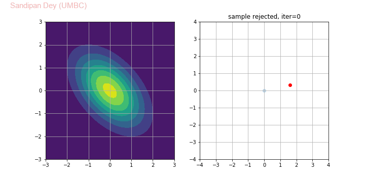
- Now, let’s try to sample from a bivariate Gaussian distribution with covariance matrix having non-zero off-diagonal entries.
mh(p_star=lambda x: multivariate_normal(mean=np.zeros(2),  \
                    cov=np.array([[1,-1/2], [-1/2,1]])).pdf(x)/10, \
                    param_init=np.zeros(2))
The following animation shows how the algorithm works.
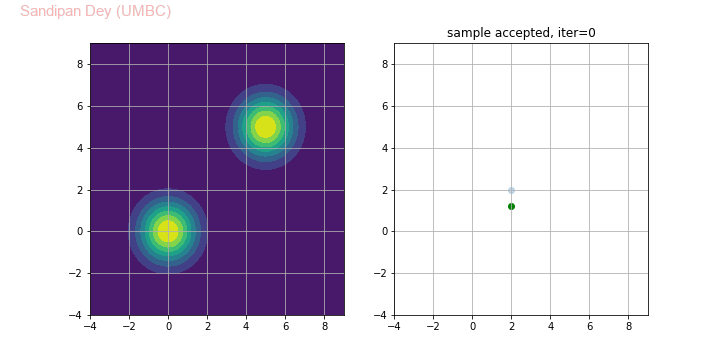
- Finally, let’s sample a bimodal distribution (mixture of 2 Gaussian) using the above algorithm using the following line of code.
def bimodal_gaussian_pdf(x):
    return multivariate_normal(mean=np.zeros(2)).pdf(x)/2 + \
           multivariate_normal(mean=5*np.ones(2)).pdf(x)/2mh(p_star=lambda x: bimodal_gaussian_pdf(x),param_init=2*np.ones(2))
The next animation shows how the samples are generated.
Bayesian Logistic Regression: Approximating the Posterior Distribution for Logistic Regression with MCMC using Metropolis-Hastings
- Let’s use the following dataset (first few records shown below) for training a logistic regression model, where the response variable is the binary variable income_more_50k and the predictor variables are age and educ, using which the model will try to predict the response.
import pandas as pd
data = pd.read_csv("adult_us_postprocessed.csv")
len(data)
#32561
data.head(20)


- First of all let’s set up a Bayesian logistic regression model (i.e. define priors on the parameters 𝛼 and 𝛽 of the model) that predicts the value of income_more_50K based on person’s age and education:

- Here 𝑥1 is a person’s age, 𝑥2 is his/her level of education, y indicates his/her level of income, 𝛼, 𝛽1 and 𝛽2 are parameters of the model which can be represented as the parameter vector θ.
- Let’s compute the posterior (upto a constant, i.e., P(θ|D) ∝ P(D|θ)P(θ)) as a product of the likelihood P(D|θ) and the prior P(θ) and use the Metropolis-Hastings algorithm to sample from the approximate (true) posterior, as shown in the following figure.

- In practice we compute log-likelihood, log-prior and log-p* to prevent numerical underflow.
- The following python code snippet shows how to compute the log-p* and also slightly modified version of the Metropolis-Hastings algorithm in order to be able to work on the log domain.
eps = 1e-12def sigmoid(x):
    return 1 / (1 + np.exp(-x))def log(x):
    x = x.copy()
    x[x <= eps] = 0
    x[x > 0] = np.log(x[x > 0])
    return xdef log_p_star(data, theta, s=100):
    y = np.array(data['income_more_50K'].tolist())
    p = sigmoid(np.dot(np.hstack((np.ones((len(data), 1)),
                 data[['age', 'educ']].to_numpy())), theta))
    return np.sum(y*log(p)+(1-y)*log(1-p)) \
           - np.dot(theta.T, theta)/2/s**2 - 3*np.log(s)def mh(log_p_star, param_init, num_samples=5000, stepsize=1.0):

theta = param_init
    samples = np.zeros((num_samples+1, param_init.shape[0]))
    samples[0] = theta
    for i in range(num_samples):
        theta_cand = multivariate_normal(mean=theta,
                     cov=[stepsize**2]*len(theta)).rvs(size=1)
        ll_cand = log_p_star(theta_cand)
        ll_old = log_p_star(theta)
        if ll_cand > ll_old:
            theta = theta_cand
        else:
            u = np.random.uniform()
            if u < np.exp(ll_cand - ll_old):
                theta = theta_cand
        samples[i+1] = theta

return samplesmh(log_p_star=lambda x: log_p_star(data, x), \
   param_init=np.random.rand(3), stepsize=0.1)
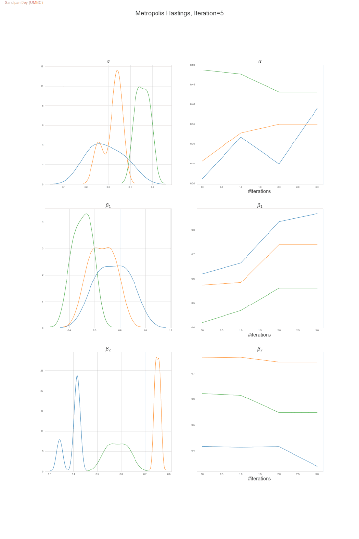
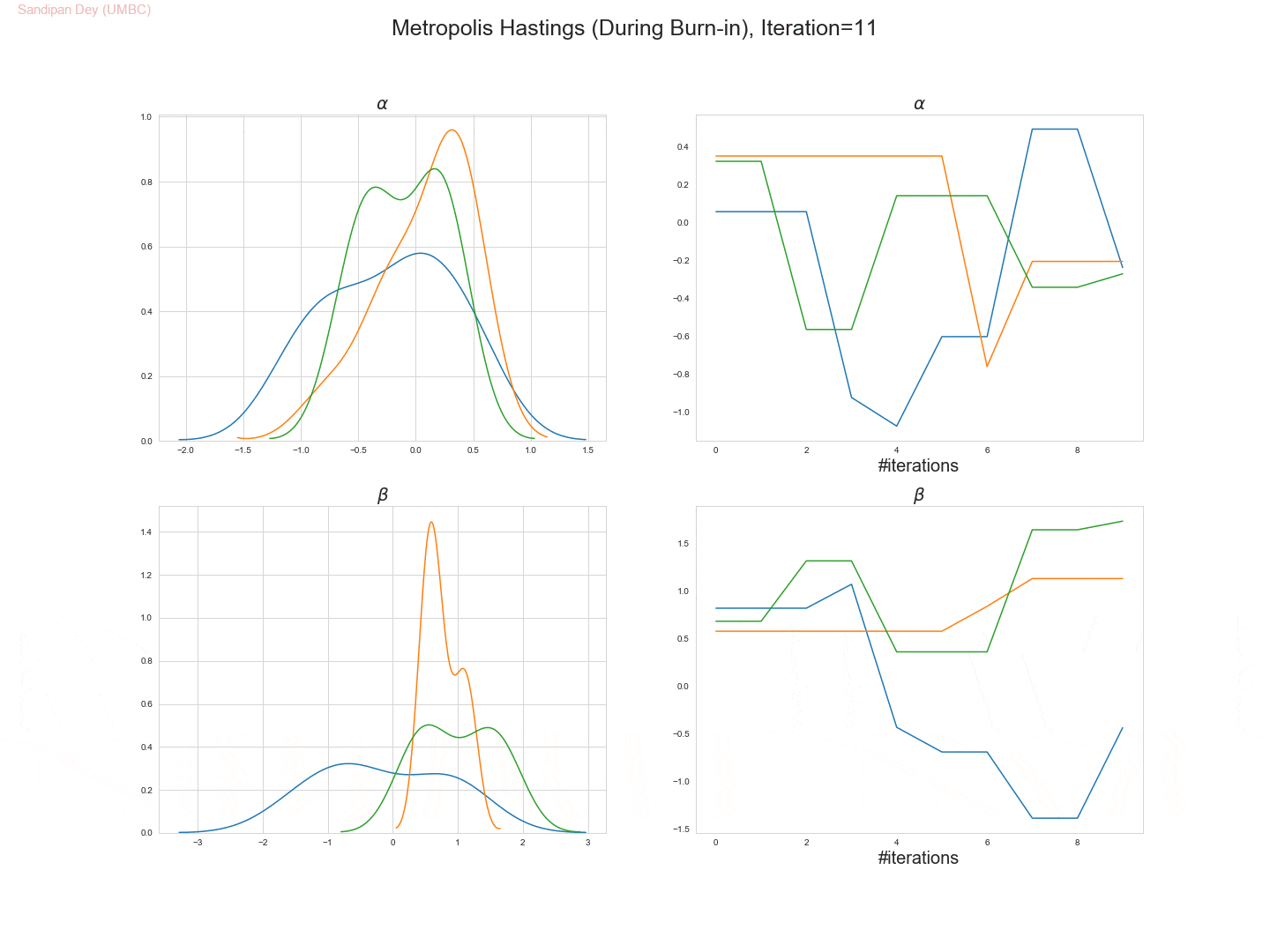
The following trace-plot animation shows how the posterior distribution is computed for each of the parameters 𝛼, 𝛽1 and 𝛽2, using 3 Markov chains corresponding to 3 different initialization of the parameters (with flat prior N(0,10000) on each of them).
Bayesian Poisson Regression
- Consider a Bayesian Poisson regression model, where outputs y_n are generated from a Poisson distribution of rate exp(α.x_n + β), where the x_n are the inputs (covariates), and α and β the parameters of the regression model for which we assume a Gaussian prior:

- We are interested in computing the posterior density of the parameters (α, β) given the data D above.
- Let’s derive and implement a function p* of the parameters α and β that is proportional to the posterior density p(α, β | D), and which can thus be used as target density in the Metropolis Hastings algorithm. For numerical accuracy, let’s perform the computation in the log domain as shown in the next figure:

- Let’s use the Metropolis Hastings algorithm to draw 5,000 samples from the posterior density p(α,β|D).
- Let’s set the (hyper-) parameters of the Metropolis-Hastings algorithm to:
• param_init= (αinit, βinit) = (0, 0),
• stepsize 1,
• number of warm-up steps W = 1000. - Let’s plot the drawn samples with x-axis α and y-axis β and report the posterior mean of α and β, as well as their correlation coefficient under the posterior.
The following python code snippet implements the algorithm:
from scipy.special import factorialdef log_p_star(x, y, theta, s=10):
    alpha, beta = theta[0], theta[1]
    x1 = np.hstack((np.ones((len(x), 1)), np.reshape(x, (-1,1))))
    sx = np.dot(x1, theta)
    return np.sum(y*sx - np.log(factorial(y)) - np.exp(sx)) - \
                 (alpha**2 + beta**2)/2/s**2 - 2*np.log(s)def mh(log_p_star, param_init, num_samples=5000, stepsize=1.0,
       warm_up=1000):

theta = param_init
    samples = np.zeros((num_samples+1, param_init.shape[0]))
    samples[0] = theta
    for i in range(num_samples):
        theta_cand = multivariate_normal(mean=theta, \
                     cov=[stepsize**2]*len(theta)).rvs(size=1)
        ll_cand = log_p_star(theta_cand)
        ll_old = log_p_star(theta)
        if ll_cand > ll_old:
            theta = theta_cand
        else:
            u = np.random.uniform()
            if u < np.exp(ll_cand - ll_old):
               theta = theta_cand
        samples[i+1] = theta    return samples[warm_up+1:]samples = mh(log_p_star=lambda theta: log_p_star(x, y, theta), \
             param_init=np.zeros(2), stepsize=1)np.mean(samples, axis=0)
# [-0.25056742,  0.91365977]np.corrcoef(samples[:,0], samples[:,1])
# [[ 1.        , -0.62391813],
   [-0.62391813,  1.        ]]
- As can be seen from above, the parameters are negatively correlated, as can also be seen from the following animation.
- The following trace plot animation shows how 3 Markov chains initialized with different parameter values converge to the stationary posteriors for the parameters.
Gibbs Sampling
Suppose x is a 2D multivariate Gaussian random variable, i.e., x ∼ N (μ, Σ), where μ = (0, 0) and Σ = (1, −0.5; −0.5, 1).
- Let’s implement Gibbs sampling to estimate the 1D marginals, p(x1) and p(x2) and plot these estimated marginals as histograms, by superimposing a plot of the exact marginals.
- In order to do Gibbs sampling, you will need the two conditionals distributions, namely, p(x1|x2) and p(x2|x1). We assume that we know how to sample from these 1D conditional (Gaussian) distributions, although we don’t know how to sample from the original 2D Gaussian.
- The following figure shows the conditional and marginal distributions for a given 2D Gaussian:

- We shall use the built-in python function numpy.random.normal() to sample from (conditional) 1D Gaussians, but we must not sample from a 2D Gaussian directly.
- The following figure describes the Gibbs sampling algorithm.

The following python code snippet shows a straightforward implementation of the above algorithm:
import numpy as npμ = np.array([0, 0])
Σ = np.array([[1, -0.5], [-0.5, 1]])μx, μy = μ[0], μ[1]
Σxx, Σyy = Σ[0,0], Σ[1,1]
Σxy = Σyx = Σ[0,1]x0, y0 = np.random.rand(), np.random.rand()N = 500
for i in range(N):
    # draw a sample from p(x | y=y0)
    x1 = np.random.normal(loc = μx + Σxy * (y0 - μy) / Σyy, \
                          scale = np.sqrt(Σxx - Σxy*Σyx/Σyy))
    # draw a sample from p(y | x=x1)
    y1 = np.random.normal(loc = μy + Σyx * (x1 - μx) / Σxx, \
                          scale = np.sqrt(Σyy - Σyx*Σxy/Σxx))
    x0, y0 = x1, y1
    #print(x1, y1)
The following animation shows how the Gibbs sampling algorithm approximates the 2D Gaussian distribution. In this case, since the 1D Gaussians are correlated, the Gibbs sampling algorithm is slow to explore the space.
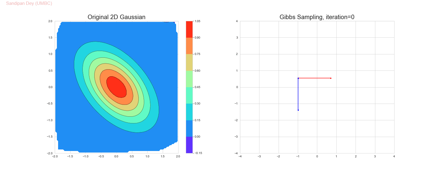
The original and the estimated marginal distributions for the random variables x and y are shown below (obtained only with 250 iterations with the Gibbs sampling algorithm):

Application in NLP: Implementing Topic Modeling with Latent Dirichlet Allocation (LDA) using collapsed Gibbs Sampling
Collapsed Gibbs sampling can be used to implement topic modeling with Latent Dirichlet allocation (LDA). Let’s first understand the Dirichlet distribution (which is a distribution of distributions) and it properties (e.g., the conjugate prior, as shown in the following figure).

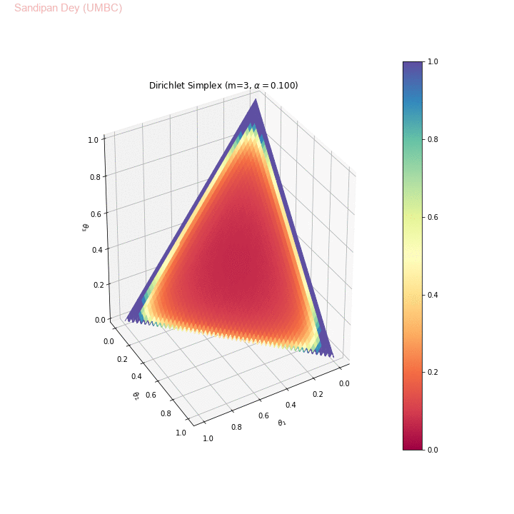
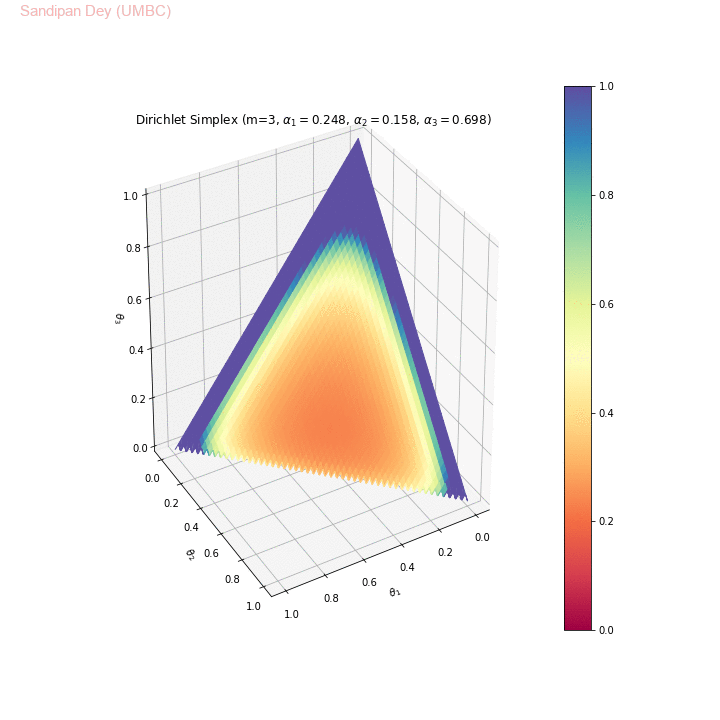
The following animation shows the Dirichlet simplex for m=3. As can be seen, for α < 1, the density gets concentrated more to the corners of the simplex, for α=1 it becomes uniform over the simplex and α > 1 the density gets concentrated more towards the center of the simplex. Here we considered the symmetric Dirichlet, i.e., α s (concentration parameter) for which α1= α2= α3 (e.g., α=(2,2,2) is denoted as α=2 in the animation). θ1, θ2 and θ3 represent 3 corners of the simplex.
The following animation shows examples of a few asymmetric Dirichlet simplices:
Latent Dirichlet Allocation (LDA)
- Each document is a (different) mixture of topics
- LDA lets each word be on a different topic
- For each document, d:
- Choose a multinomial distribution θ_d over topics for that document
- For each of the N words w_n in the document
- Choose a topic z_n with p(topic) = θ_d
- Choose a word w_n from a multinomial conditioned on z_n with p(w=w_n|topic=z_n)
- Note: each topic has a different probability of generating each word
The following figure shows the algorithm for LDA, using collapsed Gibbs Sampling:

For each of M documents in the corpus,
- Choose the topic distribution θ ~ Dirichlet(α)
- For each of the N words w_n:
- Choose a topic z ~ Multinomial(θ)
- Choose a word w_n ~ Multinomial(β_z)
Implementation To be continued…
Probabilistic Programming with PyMC3
Now, we shall learn how to use the library PyMC3 for probabilistic programming and inference.
Bayesian Logistic regression with PyMC3
- Logistic regression is a powerful model that allows us to analyze how a set of features affects some binary target label. Posterior distribution over the weights gives us an estimation of the influence of each particular feature on the probability of the target being equal to one.
- But most importantly, posterior distribution gives us the interval estimates for each weight of the model. This is very important for data analysis when we want to not only provide a good model but also estimate the uncertainty of our conclusions.
- In this problem, we will learn how to use PyMC3 library to perform approximate Bayesian inference for logistic regression (this part is based on the logistic regression tutorial by Peadar Coyle and J. Benjamin Cook).
- We shall use the same dataset as before. The problem here is to model how the probability that a person has salary ≥ $50K is affected by his/her age, education, sex and other features.
- Let y_i=1 if i-th person’s salary is ≥ $50K and y_i =0 otherwise. Let x_{ij} be the j-th feature of the i-th person.
- As explained above, the Logistic regression models this probability in the following way: p(y_i=1∣β)=σ(β1.x_{i1}+β2.x_{i2}+⋯+βk.x_{ik}), where σ(t)=1/(1+exp(−t))
Odds ratio
- Let’s try to answer the following question: does the gender of a person affects his or her salary? To do it we will use the concept of odds.
- If we have a binary random variable y (which may indicate whether a person makes $50K) and if the probabilty of the positive outcome p(y=1) is for example 0.8, we will say that the odds are 4 to 1 (or just 4 for short), because succeding is 4 time more likely than failing p(y=1)/p(y=0)=0.8/0.2=4.
- Now, let’s return to the effect of gender on the salary. Let’s compute the ratio between the odds of a male having salary ≥ $50K and the odds of a female (with the same level of education, experience and everything else) having salary ≥ $50K.
- The first feature of each person in the dataset is gender. Specifically, x_{i1}=0 if the person is female and x_{i1}=1, otherwise. Consider two people i and j having all but one features the same with the only difference in x_{i1}≠x_{j1}.
- If the logistic regression model above estimates the probabilities exactly, the odds for a male will be:

- Now the ratio of the male and female odds will be:

- So given the correct logistic regression model, we can estimate odds ratio for some feature (gender in this example) by just looking at the corresponding coefficient.
- But of course, even if all the logistic regression assumptions are met we cannot estimate the coefficient exactly from real-world data, it’s just too noisy.
- So it would be really nice to build an interval estimate, which would tell us something along the lines “with probability 0.95 the odds ratio is greater than 0.8 and less than 1.2, so we cannot conclude that there is any gender discrimination in the salaries” (or vice versa, that “with probability 0.95 the odds ratio is greater than 1.5 and less than 1.9 and the discrimination takes place because a male has at least 1.5 higher probability to get >$50k than a female with the same level of education, age, etc.”). In Bayesian statistics, this interval estimate is called credible interval.
- Unfortunately, it’s impossible to compute this credible interval analytically. So let’s use MCMC for that!
Credible interval
- A credible interval for the value of exp(β1) is an interval [a,b] such that p(a ≤ exp(β1) ≤ b ∣ Xtrain, ytrain) is 0.95 (or some other predefined value). To compute the interval, we need access to the posterior distribution p(exp(β1) ∣ Xtrain, ytrain).
- Lets for simplicity focus on the posterior on the parameters
p(β1 ∣ Xtrain, ytrain), since if we compute it, we can always find [a,b] s.t. p(loga ≤β1 ≤logb ∣ Xtrain, ytrain)= p(a ≤exp(β1) ≤b ∣ Xtrain, ytrain) = 0.95.
MAP inference
Let’s read the dataset again. This is a post-processed version of the UCI Adult dataset.
data = pd.read_csv("adult_us_postprocessed.csv")Each row of the dataset is a person with his (her) features. The last column is the target variable y, i.e., y = 1 indicates that this person’s annual salary is more than $50K.
First of all let’s set up a Bayesian logistic regression model (i.e. define priors on the parameters α and β of the model) that predicts the value of “income_more_50K” based on person’s age and education:

where x_1 is a person’s age, x_2 is his/her level of education, y indicates his/her level of income, α, β1 and β2 are parameters of the model.
with pm.Model() as manual_logistic_model:

alpha = pm.Normal('alpha', mu=0, sigma=100)
    beta1 = pm.Normal('beta1', mu=0, sigma=100)
    beta2 = pm.Normal('beta2', mu=0, sigma=100)

x1 = data.age.to_numpy()
    x2 = data.educ.to_numpy()
    z = alpha + beta1 * x1 + beta2 * x2

p = pm.invlogit(z)
    target = data.income_more_50K.to_numpy()
    y = pm.Bernoulli('income_more_50K', p=p, observed=target)

map_estimate = pm.find_MAP()
    print(map_estimate)
    # {'alpha': array(-6.74809299), 'beta1': array(0.04348244),
    #  'beta2': array(0.3621089)}
- There’s a simpler interface for generalized linear models in pyMC3. Let’s compute the MAP estimations of corresponding coefficients using it.
with pm.Model() as logistic_model:
    pm.glm.GLM.from_formula('income_more_50K ~ age + educ', data,
                            family=pm.glm.families.Binomial())
    map_estimate = pm.find_MAP()
    print(map_estimate)
    # {'Intercept': array(0.0579459), 'age': array(1.29479444),
    #  'educ': array(0.67566864)}
MCMC
To find credible regions let’s perform MCMC inference.
- Let’s use the following function to visualize the sampling process.
def plot_traces(traces, burnin=200):

ax = pm.traceplot(traces[burnin:],
                      figsize = (12,len(traces.varnames)*1.5),
                      lines={k: v['mean'] for k, v in
                            pm.summary(traces[burnin:]).iterrows()})

for i, mn in enumerate(pm.summary(traces[burnin:])['mean']):
        ax[i,0].annotate('{:.2f}'.format(mn), xy=(mn,0),
                         xycoords='data', xytext=(5,10),
                         textcoords='offset points', rotation=90,
                         va='bottom', fontsize='large',
                         color='#AA0022')
Metropolis-Hastings
- Let’s use the Metropolis-Hastings algorithm for finding the samples from the posterior distribution.
- Let’s explore the hyperparameters of Metropolis-Hastings such as the proposal distribution variance to speed up the convergence. The
plot_tracesfunction can be used to visually inspect the convergence.
We may also use MAP-estimate to initialize the sampling scheme to speed things up. This will make the warmup (burn-in) period shorter since we shall start from a probable point.
with pm.Model() as logistic_model:

pm.glm.GLM.from_formula('income_more_50K ~ age + educ', data,
                            family=pm.glm.families.Binomial())
    step = pm.Metropolis()
    trace = pm.sample(2000, step) # draw 2000 samples

plot_traces(trace)
The trace plot obtained is shown in the following figure (using 2 Markov chains, by default):

- Since it is unlikely that the dependency between the age and salary is linear, let’s now include age squared into features so that we can model dependency that favors certain ages.
- Let’s train Bayesian logistic regression model on the following features: sex, age, age², educ, hours and use pm.sample() to run MCMC to train this model, using the following code snippet:
with pm.Model() as logistic_model:

pm.glm.GLM.from_formula(
              'income_more_50K ~ sex + age + age^2 + educ + hours',
               data, family=pm.glm.families.Binomial())
    step = pm.Metropolis()
    trace = pm.sample(2000, step)plot_traces(trace)
The trace plot obtained this time is shown in the following figure:

- Now, let’s use the NUTS sampler to obtain quicker convergence, with drawing only 400 samples, using adapt_diag initialization, as shown in the next python code snippet:
with pm.Model() as logistic_model:

pm.glm.GLM.from_formula(
               'income_more_50K ~ sex + age + age^2 + educ + hours',
               data,
               family=pm.glm.families.Binomial())
    trace = pm.sample(400, init = 'adapt_diag')

- We don’t need to use a large burn-in here, since we have initialized sampling from a good point (from our approximation of the most probable
point (MAP) to be more precise).
burnin = 100
b = trace['sex[T. Male]'][burnin:]
plt.hist(np.exp(b), bins=20, density=True)
plt.xlabel("Odds Ratio")
plt.show()

- Finally, we can find a credible interval (recall that credible intervals are Bayesian and confidence intervals are frequentist) for this quantity. This may be the best part about Bayesian statistics: we get to interpret credibility intervals the way we’ve always wanted to interpret them. We are 95% confident that the odds ratio lies within our interval!
lb, ub = np.percentile(b, 2.5), np.percentile(b, 97.5)
print("P(%.3f < Odds Ratio < %.3f) = 0.95" % (np.exp(lb), np.exp(ub)))
# P(2.983 < Odds Ratio < 3.450) = 0.95
Recommend
About Joyk
Aggregate valuable and interesting links.
Joyk means Joy of geeK