Solving 1st and 2nd order ODEs with Euler method

In this article, the simplest numeric method, namely the Euler method to solve 1st order ODEs will be demonstrated with examples (and then use it to solve 2nd order ODEs). Also, we shall see how to plot the phase lines (gradient fields) for an ODE and understand from examples how to qualitatively find a solution curve with the phaselines. All the problems are taken from the edx Course: MITx — 18.03x: Introduction to Differential Equations.

Image created from the lecture notes of the edX course MITx: 18.031x (source)

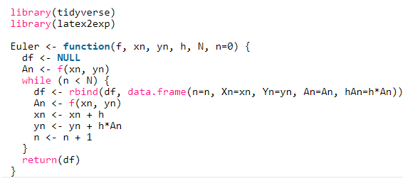
Let’s implement the above algorithm steps with the following R code snippet.

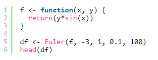
Let’s define the function f next.

The below table shows the solution curve computed by the Euler method for the first few iterations:

Image created from the lecture notes of the edX course MITx: 18.031x (source)

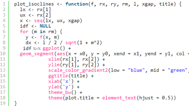
Let’s implement the following R functions to draw the isoclines and the phase lines for an ODE.

Now, let’s plot the 0 (the nullcline), 1, 2, 3 isoclines for the ODE: y’ = y.sin(x).

Image by authorImage by author

Now, let’s solve the ODE with Euler’s method, using step size h = 0.1 with the initial value y(-3) = 1.

l <- 0.2xgap <- 0.05 #05ygap <- 0.05 #05p <- plot_phaselines(f, rx, ry, xgap, ygap, l, -1:1, TeX('phaselines and m-isoclines for $\\frac{dy}{dx} = y.sin(x)$'))df <- Euler(f, -3, 1, 0.1, 100)p + geom_point(aes(Xn, Yn), data=df) + geom_path(aes(Xn, Yn), arrow = arrow(), data=df)

The black curve in the following figure shows the solution path with Euler.

Image by author

Let’s plot the phase lines for the ODE y’ = y^2 — x, solve it with Euler and plot the solution curve again, using the following code.

The black solution curve shows the trajectory of the solution obtained with Euler.

Image by author

Finally, let’ plot the isoclines for the ODE y’ = y^2 — x^2 and solve it with Euler. Let’s try starting with different initial values and observe the solution curves in each case.

f <- function(x, y) {
  return(y^2-x^2)
}rx <- c(-4,4)
ry <- c(-4,4)
l <- 0.2
xgap <- 0.1
ygap <- 0.1p <- plot_phaselines(f, rx, ry, xgap, ygap, l, -2:2, TeX('phaselines and m-isoclines for $\\frac{dy}{dx} = y^2-x^2$, solving with Euler with diff. initial values'))df <- Euler(f, -3.25, 3, 0.1, 100)
p <- p + geom_point(aes(Xn, Yn), data=df) + geom_path(aes(Xn, Yn), arrow = arrow(), data=df)

As can be seen, the solution curve starting with different initial values lead to entirely different solution paths, it depends on the phase lines and isoclines it gets trapped into.

Image by author

Finally, let’s notice the impact of the step size on the solution obtained by the Euler method, in terms of the error and the number of iterations taken to obtain the solution curve. As can be seen from the following animation, with bigger step size h=0.5, the algorithm converges to the solution path faster, but with much higher error values, particularly for the initial iterations. On the contrary, smaller step size h=0.1 taken many more iterations to converge, but the error rate is much smaller, the solution curve is pretty smooth and follows the isoclines without any zigzag movement.

Image by author

Spring-mass-dashpot system — the Damped Harmonic Oscillator

A spring is attached to a wall on its left and a cart on its right. A dashpot is attached to the cart on its left and the wall on its right. The cart has wheels and can roll either left or right.

The spring constant is labeled k, the mass is labeled m, and the damping coefficient of the dashpot is labeled b. The center of the cart is at the rest at the location x equals 0, and we take rightwards to be the positive x direction.

Consider the spring-mass-dashpot system in which mass is m (kg), and spring constant is k (Newton per meter). The position x(t) (meters) of the mass at (seconds) is governed by the DE

where m, b, k > 0. Let’s investigate the effect of the damping constant, on the solutions to the DE.

Image created from the lecture notes of the edX course MITx: 18.031x (source)

The next animation shows how the solution changes for different values of 𝑏, given 𝑚=1 and 𝑘=16, with couple of different initial values ©.

Image by author

Now, let’s observe how the amplitude of the system response increases with the increasing frequency of the input sinusoidal force, achieving the peak at resonance frequency (for m=1, k=16 and b=√14, the resonance occurs at wr = 3)

Image by author

Solving the 2nd order ODE for the damped Harmonic Oscillator with Euler method

Now, let’s see how the 2nd order ODE corresponding to the damped Harmonic oscillator system can be numerically solved using the Euler method. In order to be able to use Euler, we need to represent the 2nd order ODE as a collection of 1st order ODEs and then solve those 1st order ODEs simultaneously using Euler, as shown in the following figure:

Created from the Youtube video by Jeffrey Chasnov (source)

Let’s implement a numerical solver with Euler for a 2nd order ODE using the following R code snippet:

For the damped Harmonic Oscillator, we have the 2nd order ODE

from which we get the following two 1st order ODEs:

Let’s solve the damped harmonic oscillator with Euler method:

Now, let’s plot the solution curves using the following R code block:

par(mfrow=c(1,2))plot(df$tn, df$xn, main="x(t) vs. t", xlab='t', ylab='x(t)',  
     col='red', pch=19, cex=0.7, xaxs="i", yaxs="i")
lines(df$tn, df$xn, col='red')
grid(10, 10)plot(df$tn, df$un, main=TeX('$\\dot{x}(t)$ vs. t'), xlab='t', 
     ylab=TeX('$\\dot{x}(t)$'), col='blue', pch=19, cex=0.7, 
     xaxs="i", yaxs="i")
lines(df$tn, df$un, col='blue')
grid(10, 10)

Image by author

The following animation shows the solution curves obtained by joining the points computed with the Euler method for the damped Harmonic Oscillator:

Image by author

As can be seen from the above results, using the Euler method we can solve ODEs of any order, as long as we can represent the system as a collection of 1st order ODEs. There are more accurate methods for solving ODEs (e.g., the RK-4 method) than Euler method (also known an 1st order Runge-Kutta method) that produces much lower error in approximation (e.g., RK-4 has global error of O(h⁴)), we can use them to obtain more accurate approximation of the solution curve.