Numerical Methods with C++ Part 3: Root Approximation Algorithms

Welcome back to a new post on thoughts-on-cpp.com. This time I would like to have a closer look at root approximation methods which I regularly use to solve numerous numerical problems. We start with an easy approach using Bisection, investigating in Newton and Secant method and are concluding with black-box methods of Dekker and Brent.

Preamble

In the following chapters, we have a closer look at several algorithms used for root approximation of functions. We will compare all algorithms against the nonlinear function $f(x)=x^3-x^2-x-1$ which has only one root inside a defined range [a,b] (this criterion is quite important, otherwise it might be hard to tell which solution we got from the algorithm). An additional criteria is defined by $f(a) \cdot f(b) < 0$ . Please keep in mind that we don’t check against the number of iterations we run. This might be necessary because we usually don’t want to run infinite loops. As usual, you can find all the sources at GitHub.

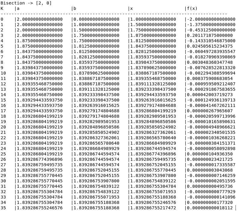
Bisection Method

Let’s start with a method which is mostly used to search for values in arrays of every size, Bisection. But it can be also used for root approximation. The benefits of the Bisection method are its implementation simplicity and its guaranteed convergence (if there is a solution, bisection will find it). The algorithm is rather simple:

Calculate the midpoint $m=\frac{a+b}{2}$ of a given interval [a,b]
Calculate the function result of midpoint m, f(m)
If new m-a or |f(m)| is fulfilling the convergence criteria we have the solution m
Comparing sign of f(m) and replace either f(a) or f(b) so that the resulting interval is including the sought root

class Bisection : public Iteration { public: Bisection(double epsilon, const std::function<double (double)> &f) : Iteration(epsilon), mf(f) {}

double solve(double a, double b) override { resetNumberOfIterations();

checkAndFixAlgorithmCriteria(a, b);

fmt::print("Bisection -> [{:}, {:}]\n", a, b); fmt::print("{:<5}|{:<20}|{:<20}|{:<20}|{:<20}\n", "K", "a", "b", "x", "f(x)"); fmt::print("———————————————————————————— \n");

double x = 0.5*(a+b); double fx = mf(x); fmt::print("{:<5}|{:<20.15f}|{:<20.15f}|{:<20.15f}|{:<20.15f}\n", incrementNumberOfIterations(), a, b, x, fx);

while(fabs(fx) >= epsilon()) { x = calculateX(x, a, b, fx); fx = mf(x);

fmt::print("{:<5}|{:<20.15f}|{:<20.15f}|{:<20.15f}|{:<20.15f}\n", incrementNumberOfIterations(), a, b, x, fx); }

fmt::print("\n");

return x; }

private: void checkAndFixAlgorithmCriteria(double &a, double &b) const { //Algorithm works in range [a,b] if criteria f(a)*f(b) < 0 and f(a) > f(b) is fulfilled assert(mf(a)*mf(b) < 0); if(mf(a) < mf(b)) { std::swap(a,b); } }

static double calculateX(double x, double &a, double &b, double fx) { if(fx >= 0) a = x; if(fx < 0) b = x;

return 0.5*(a+b); }

const std::function<double (double)> &mf; };

Implementation of Bisection Algorithm

As we can see from source code the actual implementation of Bisection is so simple that most of the code is just there to produce the output. The important part is happening inside the while loop which is executing as long as the result of f(x) is not fulfilling the criteria $f(x) < \epsilon$ . The new position x is calculated in method calculateX() which is checking the sign of f(x) and, depending on its result, assigning x to a or b to define the new range which is including the root point. Important to note is that the Bisection algorithm needs always results of f(a) and f(b) with different signs which is assured by the method checkAndFixAlgorithmCriteria(). 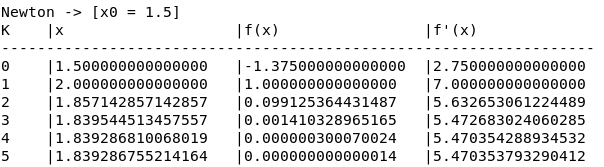The algorithm is rather slow with 36 iterations to reach the convergence criteria of $\epsilon = 1\cdot10^{-10}$ , but it will converge with enough given time, regardless what happens.

Newton Method

As long as we have also the derivative of the function and the function is smooth we can use the much faster Newton method where the next closer point to root $x_{n+1}$ can be calculated by:

$x_{n+1}=x_n-\frac{f(x_n)}{f'(x_n)}$

class Newton : public Iteration { public: Newton(double epsilon, const std::function<double (double)> &f, const std::function<double (double)> &fPrime) : Iteration(epsilon), mf(f), mfPrime(fPrime) {}

double solve(double x) override { resetNumberOfIterations();

fmt::print("Newton -> [x0 = {:}]\n", x); fmt::print("{:<5}|{:<20}|{:<20}|{:<20}\n", "K", "x", "f(x)", "f'(x)"); fmt::print("—————————————————————— \n");

double fx = mf(x); double fxPrime = mfPrime(x); fmt::print("{:<5}|{:<20.15f}|{:<20.15f}|{:<20.15f}\n", incrementNumberOfIterations(), x, fx, fxPrime);

while(fabs(fx) >= epsilon()) { x = calculateX(x, fx, fxPrime);

fx = mf(x); fxPrime = mfPrime(x);

fmt::print("{:<5}|{:<20.15f}|{:<20.15f}|{:<20.15f}\n", incrementNumberOfIterations(), x, fx, fxPrime); }

fmt::print("\n");

return x; }

private: static double calculateX(double x, double fx, double fxPrime) { assert(fabs(fxPrime) >= std::numeric_limits<double>::min());

return x – fx/fxPrime; }

const std::function<double (double)> &mf; const std::function<double (double)> &mfPrime; };

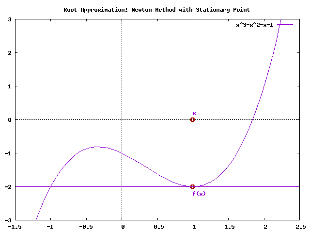
Implementation of Newton Algorithm

Also this algorithm is iterating as long as the result of f(x) is not fulfilling the criteria $f(x) < \epsilon$ . The method calculateX() is not only applying the formula of the Newton method, but it is also checking if the derivative of f(x) is getting zero. Because floating point numbers can’t be compared directly we have to compare f'(x) against the smallest possible floating point number close to zero which we can get by calling std::numeric_limits<double>::min(). In such a case, where f'(x) is zero, the algorithm wouldn’t be able to converge (stationary point) as shown in the image below.

Newton algorithm with stationary condition

The advantage of the Newton method is its raw speed. In our case it just needs 6 iterations until the algorithm is reaching the convergence criteria of $\epsilon = 1\cdot10^{-10}$ . But the algorithm has also several drawbacks as implied above. Such as:

Only suitable if we know the derivative of a given function
Only suitable for smooth and continuously functions
If starting point $x_0$ is chosen wrong or the calculated point $x_{n+1}$ at or close to a local maximum or minimum, the derivative of f'(x) gets 0 and we have a stationary point condition.
If the derivative of a function is not well behaving, the Newton method tends to overshoot. Then $x_{n+1}$ might be way to far from root to be useful to the algorithm

Secant Method

In many cases, we don’t have, or it might be to complex, a derivative of a function f(x). In such cases, we can use the Secant method. This method is doing basically the same as the Newton method, but calculating the necessary slope not via its function derivative f'(x) but through the quotient of two x and y values calculated with f(x).

$x_{n+1}=x_n-f(x_n)\frac{x_n-x_{n-1}}{f(x_n)-f(x_{n-1})}$

class Secant : public Iteration { public: Secant(double epsilon, const std::function<double (double)> &f) : Iteration(epsilon), mf(f) {}

double solve(double a, double b) override { resetNumberOfIterations();

fmt::print("Secant -> [{:}, {:}]\n", a, b); fmt::print("{:<5}|{:<20}|{:<20}|{:<20}|{:<20}\n", "K", "a", "b", "f(a)", "f(b)"); fmt::print("————————————————————————————–\n");

if(mf(a) > mf(b)) { std::swap(a,b); }

double x = b; double lastX = a; double fx = mf(b); double lastFx = mf(a);

fmt::print("{:<5}|{:<20.15f}|{:<20.15f}|{:<20.15f}|{:<20.15f}\n", incrementNumberOfIterations(), x, lastX, fx, lastFx);

while(fabs(fx) >= epsilon()) { const double x_tmp = calculateX(x, lastX, fx, lastFx);

lastFx = fx; lastX = x; x = x_tmp;

fx = mf(x);

fmt::print("{:<5}|{:<20.15f}|{:<20.15f}|{:<20.15f}|{:<20.15f}\n", incrementNumberOfIterations(), x, lastX, fx, lastFx); }

fmt::print("\n");

return x; }

private: static double calculateX(double x, double lastX, double fx, double lastFx) { const double functionDifference = fx – lastFx; assert(fabs(functionDifference) >= std::numeric_limits<double>::min());

return x – fx*(x-lastX)/functionDifference; }

const std::function<double (double)> &mf; };

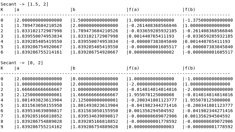
Implementation of Secant Algorithm

This algorithm needs a range [a,b] which might include (not absolutely necessary but it helps) the root we are searching for. It is using the method calculateX() is not only calculating 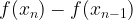$x_{n+1}$ , its also checking if the denominator $f(x_n)-f(x_{n-1})$ is 0. Also, this algorithm is very fast, it needs only 7 iterations in a well-chosen range and 10 iterations in a broader range. Both calculations are fulfilling the same convergence criteria of $\epsilon = 1\cdot10^{-10}$ . As well as the Newton method this algorithm has also its drawbacks which we have to be aware of:

Only suitable for smooth and continuously functions
If one of the calculated points $x_{n+1}$ at or close to a local maximum or minimum, the derivative of f'(x) gets 0 and we have a stationary point condition.
If the calculated slope quotient of a function has a very low steepness, also the Secant method tends to overshoot. Then $x_{n+1}$ might be way to far from root to be useful to the algorithm
If the range [a,b] is chosen wrong, e.g. including local minimum and maximum, the algorithm tends to oscillation. In general minimum and maximum, local or global, are in some cases a problem for the Secant method

Dekker Method

The idea of Dekker’s method is now to combine the speed of the Newton/Secant method with the convergence guarantee of Bisection. The algorithm is defined as the following:

$s=\left\{ \begin{matrix} b_k-f(b_k)\frac{b_k-b_{k-1}}{f(b_k)-f(b_{k-1})}, & if \: f(b_k) \neq f(b_{k-1}) \\ m & otherwise \end{matrix} \quad \right.$

$m=\frac{a+b}{2}$

$b_k$ is the current iteration guess of the root and $a_k$ is the current counterpoint of $b_k$ such that $f(a_k)$ and $f(b_k)$ have opposite signs.
The algorithm has to fulfill the criteria $f(b_k) \leq f(a_k)$ such that $b_k$ is the closest solution to the root
$f(b_{k-1})$ is the last iteration value, starting with $b_{k-1}=a_k$ at the beginning of the algorithm
If s is between m and $b_k$ then $b_{k+1}=s$ , otherwise $b_{k+1}=m$
If $f(a_k)f(b_{k+1}) > 0 \wedge f(b_k)f(b_{k+1}) < 0$ then $a_{k+1} = b_k$ otherwise $a_{k+1} = a_k$

class Dekker : public Iteration { public: Dekker(double epsilon, const std::function<double (double)> &f) : Iteration(epsilon), mf(f) {}

double solve(double a, double b) override { resetNumberOfIterations();

double fa = mf(a); double fb = mf(b);

checkAndFixAlgorithmCriteria(a, b, fa, fb);

fmt::print("Dekker -> [{:}, {:}]\n", a, b); fmt::print("{:<5}|{:<20}|{:<20}|{:<20}|{:<20}\n", "K", "a", "b", "f(a)", "f(b)"); fmt::print("———————————————————————————— \n"); fmt::print("{:<5}|{:<20.15f}|{:<20.15f}|{:<20.15f}|{:<20.15f}\n", incrementNumberOfIterations(), a, b, fa, fb);

double lastB = a; double lastFb = fa;

while(fabs(fb) > epsilon() && fabs(b-a) > epsilon()) { const double s = calculateSecant(b, fb, lastB, lastFb); const double m = calculateBisection(a, b);

lastB = b;

b = useSecantMethod(b, s, m) ? s : m;

lastFb = fb; fb = mf(b);

if (fa * fb > 0 && fb * lastFb < 0) { a = lastB; }

fa = mf(a); checkAndFixAlgorithmCriteria(a, b, fa, fb);

fmt::print("{:<5}|{:<20.15f}|{:<20.15f}|{:<20.15f}|{:<20.15f}\n", incrementNumberOfIterations(), a, b, fa, fb); }

fmt::print("\n");

return b; }

private: static void checkAndFixAlgorithmCriteria(double &a, double &b, double &fa, double &fb) { //Algorithm works in range [a,b] if criteria f(a)*f(b) < 0 and f(a) > f(b) is fulfilled assert(fa*fb < 0); if (fabs(fa) < fabs(fb)) { std::swap(a, b); std::swap(fa, fb); } }

static double calculateSecant(double b, double fb, double lastB, double lastFb) { //No need to check division by 0, in this case the method returns NAN which is taken care by useSecantMethod method return b-fb*(b-lastB)/(fb-lastFb); }

static double calculateBisection(double a, double b) { return 0.5*(a+b); }

static bool useSecantMethod(double b, double s, double m) { //Value s calculated by secant method has to be between m and b return (b > m && s > m && s < b) || (b < m && s > b && s < m); }

const std::function<double (double)> &mf; };

Implementation of Dekker Algorithm

As we can see in the implementation of Dekker’s method we always calculate both values, m and s, with the methods calculateSecant() and calculateBisection() and assigning the results depending onto what the method useSecantMethod() is confirming if s is between m and $b_k$ (as in rule 4 defined). In line 32-33 we confirm if the resulting values of the function f(x) are fulfilling rule number 5. Because of the Bisection, we have to check and correct after each iteration if the condition of $latex f(a_k)f(b_k) < 0 &s=1 & is still accomplished which is done with the method checkAndFixAlgorithmCriteria().

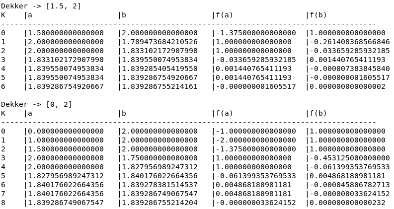
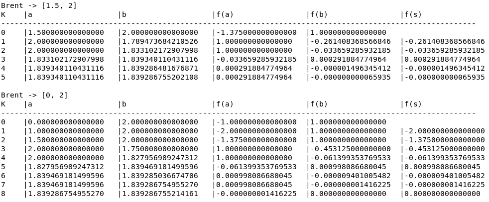
The Dekker algorithm is as fast as the Newton/Secant method but also guarantees convergence. It takes 7 iterations in case of a well-chosen range and 9 iterations in case of a broader range. As we can see the Dekker algorithm is very fast but there are examples where $|b_k-b_{k+1}|$ is extremely small but is still using the secant method. In such cases, the algorithm will take even more iterations as the pure Bisection would take.

Brent Method

Because of Dekker’s slow convergence problem, the method was extended by Brent which is now known as Brent’s method or Brent-Dekker-Method. This algorithm is extending Dekker’s algorithm by using four points (a, b, $b_{k-1}$ and $b_{k-2}$ ) instead of just three points, additional Inverse Quadratic Interpolation instead of just linear interpolation and Bisection, and additional conditions to prevent slow convergence. The algorithm decides with the following conditions which of the methods to use, Bisection, Secant method or Inverse Quadratic Interpolation:

Bisection (B = last iteration was using Bisection)
- $B \wedge |s-b_k| \geq (b_k-b_{k-1})/2$ $!B \wedge |s-b_k| \geq (b_{k-1}-b_{k-2})/2$ $B \wedge |b_k-b_{k-1}|< |\delta|$ $!B \wedge |b_{k-1}-b_{k-2}|< |\delta|$
Inverse Quadratic Interpolation
- $f(a_k) \neq f(b_{k-1}) \wedge f(b_k) \neq f(b_{k-1})$
In all other cases use the Secant method

class Brent : public Iteration { public: Brent(double epsilon, const std::function<double (double)> &f) : Iteration(epsilon), mf(f) {}

double solve(double a, double b) override { resetNumberOfIterations();

double fa = mf(a); double fb = mf(b);

checkAndFixAlgorithmCriteria(a, b, fa, fb);

fmt::print("Brent -> [{:}, {:}]\n", a, b); fmt::print("{:<5}|{:<20}|{:<20}|{:<20}|{:<20}|{:<20}\n", "K", "a", "b", "f(a)", "f(b)", "f(s)"); fmt::print("———————————————————————————————————- \n"); fmt::print("{:<5}|{:<20.15f}|{:<20.15f}|{:<20.15f}|{:<20.15f}\n", incrementNumberOfIterations(), a, b, fa, fb, "");

double lastB = a; // b_{k-1} double lastFb = fa; double s = std::numeric_limits<double>::max(); double fs = std::numeric_limits<double>::max(); double penultimateB = a; // b_{k-2}

bool bisection = true; while(fabs(fb) > epsilon() && fabs(fs) > epsilon() && fabs(b-a) > epsilon()) { if(useInverseQuadraticInterpolation(fa, fb, lastFb)) { s = calculateInverseQuadraticInterpolation(a, b, lastB, fa, fb, lastFb); } else { s = calculateSecant(a, b, fa, fb); }

if(useBisection(bisection, a, b, lastB, penultimateB, s)) { s = calculateBisection(a, b); bisection = true; } else { bisection = false; }

fs = mf(s); penultimateB = lastB; lastB = b;

if(fa*fs < 0) { b = s; } else { a = s; }

fa = mf(a); lastFb = fb; fb = mf(b); checkAndFixAlgorithmCriteria(a, b, fa, fb);

fmt::print("{:<5}|{:<20.15f}|{:<20.15f}|{:<20.15f}|{:<20.15f}|{:<20.15f}\n", incrementNumberOfIterations(), a, b, fa, fb, fs); }

fmt::print("\n");

return fb < fs ? b : s; }

private: static double calculateBisection(double a, double b) { return 0.5*(a+b); }

static double calculateSecant(double a, double b, double fa, double fb) { //No need to check division by 0, in this case the method returns NAN which is taken care by useSecantMethod method return b-fb*(b-a)/(fb-fa); }

static double calculateInverseQuadraticInterpolation(double a, double b, double lastB, double fa, double fb, double lastFb) { return a*fb*lastFb/((fa-fb)*(fa-lastFb)) + b*fa*lastFb/((fb-fa)*(fb-lastFb)) + lastB*fa*fb/((lastFb-fa)*(lastFb-fb)); }

static bool useInverseQuadraticInterpolation(double fa, double fb, double lastFb) { return fa != lastFb && fb != lastFb; }

static void checkAndFixAlgorithmCriteria(double &a, double &b, double &fa, double &fb) { //Algorithm works in range [a,b] if criteria f(a)*f(b) < 0 and f(a) > f(b) is fulfilled assert(fa*fb < 0); if (fabs(fa) < fabs(fb)) { std::swap(a, b); std::swap(fa, fb); } }

bool useBisection(bool bisection, double a, double b, double lastB, double penultimateB, double s) const { static const double DELTA = epsilon() + std::numeric_limits<double>::min();

return (bisection && fabs(s-b) >= 0.5*fabs(b-lastB)) || //Bisection was used in last step but |s-b|>=|b-lastB|/2 <- Interpolation step would be to rough, so still use bisection (!bisection && fabs(s-b) >= 0.5*fabs(lastB-penultimateB)) || //Interpolation was used in last step but |s-b|>=|lastB-penultimateB|/2 <- Interpolation step would be to small (bisection && fabs(b-lastB) < DELTA) || //If last iteration was using bisection and difference between b and lastB is < delta use bisection for next iteration (!bisection && fabs(lastB-penultimateB) < DELTA); //If last iteration was using interpolation but difference between lastB ond penultimateB is < delta use biscetion for next iteration }

const std::function<double (double)> &mf; };

Implementation of Brent Algorithm

With these modifications, the Brent algorithm is at least as fast as Bisection but in best cases slightly faster than using the pure Secant method. The Brent algorithm takes 6 iterations in case of a well-chosen range and 9 iterations in case of a broader range.

But which algorithm to chose?

We have seen five different algorithms we can use to approximate the root of a function, Bisection, Newton Method, Secant Method, Dekker, and Brent. All of them have different possibility and drawbacks. In general, we could argue which algorithm to use as the following:

Use the Newton method in case of smooth and wel- behaving functions where you have also the function’s derivative
Use the Secant method in case of smooth and well-behaving functions where you don’t have the function’s derivative
Use the Brent method in cases where you’re not sure or know your functions have jumps or other problems.

AlgorithmStart/RangeNo. Of IterationsBisection[0, 2]36Newtonx0 = 1.56Secant Good[1.5, 2]7Secant Bad[0, 2] 10Dekker Good[1.5, 2] 7Dekker Bad[0, 2] 9Brent Good[1.5, 2] 6Brent Bad[0, 2] 9

Did you like the post?
What are your thoughts? Did you like the post?
Feel free to comment and share this post.

Please also join my mailing list, seldom mails, no spam and no advertising, guaranteed.
By clicking submit, you agree to share your email address with the site owner and Mailchimp to receive updates, and other emails from the site owner. Use the unsubscribe link in those emails to opt out at any time.

Preamble

Bisection Method

Newton Method

Secant Method

Dekker Method

Brent Method

But which algorithm to chose?

Recommend

Something about backformation or analogy to vendor prefixed APIs.

CPP 3.0：从课题组到科技公司

(Relationally) Comparing Strings in JavaScript, WebMaster edition

For the love of all that's holy, please progressively enhance modal "downlo...

Speaking Machine and Human in the Second Machine Age

Anonymous table box creation and Google Plus Mobile

User Agent Switcher XML file

招募公告 | CPPers，我们在等你！

Thanks Google?

More than anyone needs to know about word-break colon break-word.

About Joyk