

A small adjustment to the Poisson model that improves predictions.
source link: http://opisthokonta.net/?p=1701
Go to the source link to view the article. You can view the picture content, updated content and better typesetting reading experience. If the link is broken, please click the button below to view the snapshot at that time.

A small adjustment to the Poisson model that improves predictions.
There are a lot extensions to the basic Poisson model for predicting football results, where perhaps the most popular is the Dixon-Coles model which I and other have written a lot about. One paper that seem to have received little attention is the 2001 paper Prediction and Retrospective Analysis of Soccer Matches in a League by Håvard Rue and Øyvind Salvesen (preprint available here). The model they describe in the paper extend the Dixon-Coles and Poisson model in several ways. The most interesting extension in how they allow the attack and defense parameters vary over time, by estimating a separate set of parameters for each match. This might at first seem like a task that should be impossible, but they manage to pull it of by using some Bayesian magic that let the estimated parameters borrow information across time. I have tried to implement something similar like this in Stan, but I haven’t gotten it to work quite right, so that will have to wait for another time. There’s many other interesting extensions in the paper as well, and here I am going to focus on one of of them which is an adjustment for teams to over and underestimate opponents when they differ in strengths.
The adjustment is added to the formulas for calculating the log-expected goals. So if team A plays team B at home, the log-expected goals \lambda_A and \lambda_B
\lambda_A = \alpha + \beta + attack_{A} – defense_{B} – \gamma \Delta_{AB}\lambda_B = \alpha + attack_{B} – defense_{A} + \gamma \Delta_{AB}
In these formulas are \alpha the intercept, \beta the home team advantage and \Delta_{AB} is a factor that determines the amount a team under- or overestimation the strength of the opponent. This factor is given as
\Delta_{AB} = (attack_{A} + defense_{A} – attack_{B} – defense_{B}) / 2The parameter \gamma determines how large this effect is. A positive \gamma implies that a strong team will underestimate a weak opponent, and thereby score fewer goals than we would otherwise expect, and vice versa for the opponent.
In the paper they do not estimate the \gamma parameter directly together with the other parameters, but instead set it to a constant, with a value they determine by backtesting to maximize predictive ability.
When I implemented this model in R and estimated it using Maximum Likelihood I noticed that adding the adjustment did not improve the model fit. I suspect that this might be because the model is nearly unidentifiable. I even tried to add a Normal prior on \gamma and get a Maximum a Posteriori (MAP) estimate, but then the MAP estimate were completely determined by the expected value of the prior. Because of these problems I decided to use a different strategy: I estimated the model without the adjustment, but add the adjustment when making predictions.
I am not going to post any R code on how to do this, but if you have estimated a Poisson or Dixon-Coles model, it should not be that difficult to add the adjustment when you calculate the predictions. If you are going to use some of the code I have posted on this blog before, you should notice the important detail that in the formulation above I have followed the paper and changed the signs of the defense parameters.
In the paper Rue and Salvesen write that \gamma = 0.1 seemed to be an overall good value when they analyze English Premier League data. To see if my approach of adding the adjustment only when doing predictions is reasonable I did a leave-one-out cross validation on some seasons of English Premier League and German Bundesliga. I fitted the model to all the games in a season, except one, and then add the adjustment when predicting the result of the left out match. I did this for several values of \gamma to see which values works best.
Here is a plot of the Ranked Probability Score (RPS), which is a measure of prediction accuracy, against different values of \gamma for the 2011-12 Premier League season:
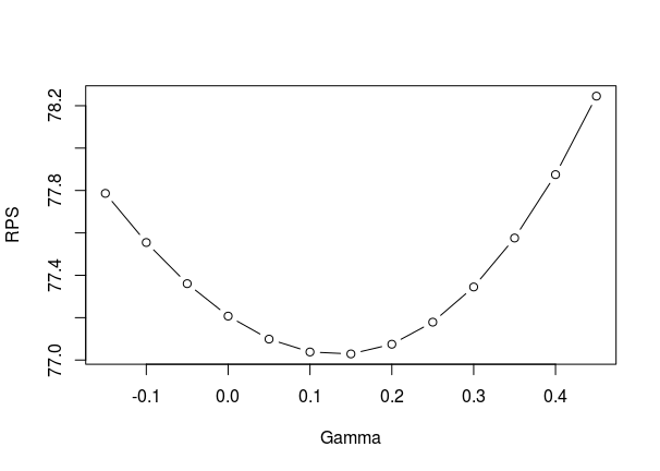
As you see I even tried some negative values of \gamma, just in case. At least in this season the result agrees with the estimate \gamma = 0.1 that Rue and Salvesen reported. In some of the later seasons that I checked the optimal \gamma varies somewhat. In some seasons it is almost 0, but then again in some others it is around 0.1. So at least for Premier league, using \gamma = 0.1 seems reasonable.
Things are a bit different in Bundesliga. Here is the same kind of plot for the 2011-12 season:

As you see the optimal value here is around 0.25. In the other seasons I checked the optimal value were somewhere between 0.15 and 0.3. So the effect of over- and underestimating the opponent seem to be greater in the Bundesliga than in Premier League.
Recommend
-
28
-
11
Underdispersed Poisson alternatives seem to be better at predicting football results Posted on August 24, 2015 In the
-
17
The Dixon-Coles approach to time-weighted Poisson regression Posted on January 19, 2015 In the previous blog posts about predicting football results using Poisson...
-
7
Predicting football results with Poisson regression pt. 2 Posted on March 7, 2013 In part 1 I wrote about the basics o...
-
10
Use poisson rather than regress; tell a friend Do you ever fit regressions of the form ln(yj) = b0 + b1x1j + b2x2j + … + bkxkj + εj
-
7
Notes on Poisson Regression Notes on Poisson Regression By Andrew Wheeler Introduction These are lecture notes on Poisson regression. It goes through how to interpret the Poisson distribution, fitting P...
-
8
July 5, 2021If you aren't used to staring at math, Poisson's equation looks a little intimidating: ∇2f=h What does ∇2f even mean? What is h? Why should I care? In this post I'll walk you through what it mea...
-
31
ICRA 2021|用于LiDAR里程计和建图的Poisson表面重建 Original...
-
2
October 20, 2021
-
4
Tesla bumps up Model Y price after EV tax credit adjustment / The Model Y’s sticker price is no longer bridled by the government’s $55,000 cap to qualify for EV tax credits.By
About Joyk
Aggregate valuable and interesting links.
Joyk means Joy of geeK