I’m using Spotify since 2013 as the main source of music, and back at that time the app automatically created a playlist for songs that I liked from artists’ radios. By innertion I’m still using the playlist to save songs that I like. As the playlist became a bit big and a bit old (6 years, huh), I’ve decided to try to analyze it.

Boring preparation

To get the data I used Spotify API and spotipy as a Python client. I’ve created an application in the Spotify Dashboard and gathered the credentials. Then I was able to initialize and authorize the client:

import spotipy
import spotipy.util as util

token = util.prompt_for_user_token(user_id,
                                   'playlist-read-collaborative',
                                   client_id=client_id,
                                   client_secret=client_secret,
                                   redirect_uri='http://localhost:8000/')
sp = spotipy.Spotify(auth=token)

Tracks metadata

As everything is inside just one playlist, it was easy to gather. The only problem was that user_playlist method in spotipy doesn’t support pagination and can only return the first 100 track, but it was easily solved by just going down to private and undocumented _get:

playlist = sp.user_playlist(user_id, playlist_id)
tracks = playlist['tracks']['items']
next_uri = playlist['tracks']['next']
for _ in range(int(playlist['tracks']['total'] / playlist['tracks']['limit'])):
    response = sp._get(next_uri)
    tracks += response['items']
    next_uri = response['next']

tracks_df = pd.DataFrame([(track['track']['id'],
                           track['track']['artists'][0]['name'],
                           track['track']['name'],
                           parse_date(track['track']['album']['release_date']) if track['track']['album']['release_date'] else None,
                           parse_date(track['added_at']))
                          for track in playlist['tracks']['items']],
                         columns=['id', 'artist', 'name', 'release_date', 'added_at'] )

tracks_df.head(10)

The first naive idea of data to get was the list of the most appearing artists:

tracks_df \
    .groupby('artist') \
    .count()['id'] \
    .reset_index() \
    .sort_values('id', ascending=False) \
    .rename(columns={'id': 'amount'}) \
    .head(10)

But as taste can change, I’ve decided to get top five artists from each year and check if I was adding them to the playlist in other years:

counted_year_df = tracks_df \
    .assign(year_added=tracks_df.added_at.dt.year) \
    .groupby(['artist', 'year_added']) \
    .count()['id'] \
    .reset_index() \
    .rename(columns={'id': 'amount'}) \
    .sort_values('amount', ascending=False)

in_top_5_year_artist = counted_year_df \
    .groupby('year_added') \
    .head(5) \
    .artist \
    .unique()

counted_year_df \
    [counted_year_df.artist.isin(in_top_5_year_artist)] \
    .pivot('artist', 'year_added', 'amount') \
    .fillna(0) \
    .style.background_gradient()

year_added 2013 2014 2015 2016 2017 2018 2019 artist Arcade Fire 2 0 0 1 3 0 0 Clinic 1 0 0 2 0 0 1 Crystal Castles 0 0 2 2 0 0 0 Depeche Mode 1 0 3 1 0 2 0 Die Antwoord 1 4 0 0 0 1 0 FM Belfast 3 3 0 0 0 0 0 Factory Floor 3 0 0 0 0 0 0 Fever Ray 3 1 1 0 1 0 0 Grimes 1 0 3 1 0 0 0 Holy Ghost! 1 0 0 0 3 1 1 Joe Goddard 0 0 0 0 3 1 0 John Maus 0 0 4 0 0 0 1 KOMPROMAT 0 0 0 0 0 0 2 LCD Soundsystem 0 0 1 0 3 0 0 Ladytron 5 1 0 0 0 1 0 Lindstrøm 0 0 0 0 0 0 2 Marie Davidson 0 0 0 0 0 0 2 Metronomy 0 1 0 6 0 1 1 Midnight Magic 0 4 0 0 1 0 0 Mr. Oizo 0 0 0 1 0 3 0 New Order 1 5 0 0 0 0 0 Pet Shop Boys 0 12 0 0 0 0 0 Röyksopp 0 4 0 3 0 0 0 Schwefelgelb 0 0 0 0 1 0 4 Soulwax 0 0 0 0 5 3 0 Talking Heads 0 0 3 0 0 0 0 The Chemical Brothers 0 0 2 0 1 0 3 The Fall 0 0 0 0 0 2 0 The Knife 5 1 3 1 0 0 1 The Normal 0 0 0 2 0 0 0 The Prodigy 0 0 0 0 0 2 0 Vitalic 0 0 0 0 2 2 0

As a bunch of artists was reappearing in different years, I decided to check if that correlates with new releases, so I’ve checked the last ten years:

counted_release_year_df = tracks_df \
    .assign(year_added=tracks_df.added_at.dt.year,
            year_released=tracks_df.release_date.dt.year) \
    .groupby(['year_released', 'year_added']) \
    .count()['id'] \
    .reset_index() \
    .rename(columns={'id': 'amount'}) \
    .sort_values('amount', ascending=False)

counted_release_year_df \
    [counted_release_year_df.year_released.isin(
        sorted(tracks_df.release_date.dt.year.unique())[-11:]
    )] \
    .pivot('year_released', 'year_added', 'amount') \
    .fillna(0) \
    .style.background_gradient()

year_added 2013 2014 2015 2016 2017 2018 2019 year_released 2010.0 19 8 2 10 6 5 10 2011.0 14 10 4 6 5 5 5 2012.0 11 15 6 5 8 2 0 2013.0 28 17 3 6 5 4 2 2014.0 0 30 2 1 0 10 1 2015.0 0 0 15 5 8 7 9 2016.0 0 0 0 8 7 4 5 2017.0 0 0 0 0 23 5 5 2018.0 0 0 0 0 0 4 8 2019.0 0 0 0 0 0 0 14

Audio features

Spotify API has an endpoint that provides features like danceability, energy, loudness and etc for tracks. So I gathered features for all tracks from the playlist:

features = []
for n, chunk_series in tracks_df.groupby(np.arange(len(tracks_df)) // 50).id:
    features += sp.audio_features([*map(str, chunk_series)])
features_df = pd.DataFrame.from_dict(filter(None, features))
tracks_with_features_df = tracks_df.merge(features_df, on=['id'], how='inner')

tracks_with_features_df.head()

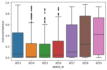
After that I’ve checked changes in features over time, only instrumentalness had some visible difference:

sns.boxplot(x=tracks_with_features_df.added_at.dt.year,
            y=tracks_with_features_df.instrumentalness)

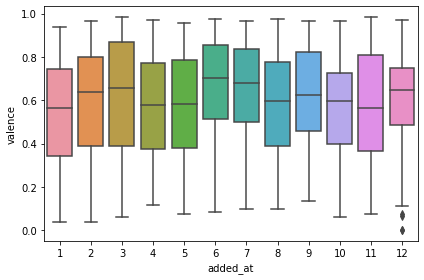
Then I had an idea to check seasonality and valence, and it kind of showed that in depressing months valence is a bit lower:

sns.boxplot(x=tracks_with_features_df.added_at.dt.month,
            y=tracks_with_features_df.valence)

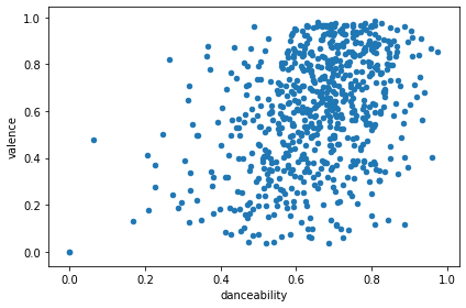
To play a bit more with data, I decided to check that danceability and valence might correlate:

tracks_with_features_df.plot(kind='scatter', x='danceability', y='valence')

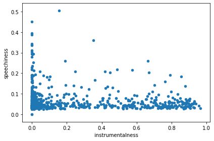
And to check that the data is meaningful, I checked instrumentalness vs speechiness, and those featues looked mutually exclusive as expected:

tracks_with_features_df.plot(kind='scatter', x='instrumentalness', y='speechiness')

Tracks difference and similarity

As I already had a bunch of features classifying tracks, it was hard not to make vectors out of them:

encode_fields = [
    'danceability',
    'energy',
    'key',
    'loudness',
    'mode',
    'speechiness',
    'acousticness',
    'instrumentalness',
    'liveness',
    'valence',
    'tempo',
    'duration_ms',
    'time_signature',
]

def encode(row):
    return np.array([
        (row[k] - tracks_with_features_df[k].min())
        / (tracks_with_features_df[k].max() - tracks_with_features_df[k].min())
        for k in encode_fields])

tracks_with_features_encoded_df = tracks_with_features_df.assign(
    encoded=tracks_with_features_df.apply(encode, axis=1))

Then I just calculated distance between every two tracks:

tracks_with_features_encoded_product_df = tracks_with_features_encoded_df \
    .assign(temp=0) \
    .merge(tracks_with_features_encoded_df.assign(temp=0), on='temp', how='left') \
    .drop(columns='temp')
tracks_with_features_encoded_product_df = tracks_with_features_encoded_product_df[
    tracks_with_features_encoded_product_df.id_x != tracks_with_features_encoded_product_df.id_y
]
tracks_with_features_encoded_product_df['merge_id'] = tracks_with_features_encoded_product_df \
    .apply(lambda row: ''.join(sorted([row['id_x'], row['id_y']])), axis=1)
tracks_with_features_encoded_product_df['distance'] = tracks_with_features_encoded_product_df \
    .apply(lambda row: np.linalg.norm(row['encoded_x'] - row['encoded_y']), axis=1)

After that I was able to get most similar songs/songs with the minimal distance, and it selected kind of similar songs:

tracks_with_features_encoded_product_df \
    .sort_values('distance') \
    .drop_duplicates('merge_id') \
    [['artist_x', 'name_x', 'release_date_x', 'artist_y', 'name_y', 'release_date_y', 'distance']] \
    .head(10)

The most different songs weren’t that fun, as two songs were too different from the rest:

tracks_with_features_encoded_product_df \
    .sort_values('distance', ascending=False) \
    .drop_duplicates('merge_id') \
    [['artist_x', 'name_x', 'release_date_x', 'artist_y', 'name_y', 'release_date_y', 'distance']] \
    .head(10)

Then I calculated the most avarage songs, eg the songs with the least distance from every other song:

tracks_with_features_encoded_product_df \
    .groupby(['artist_x', 'name_x', 'release_date_x']) \
    .sum()['distance'] \
    .reset_index() \
    .sort_values('distance') \
    .head(10)

And totally opposite thing – the most outstanding songs:

tracks_with_features_encoded_product_df \
    .groupby(['artist_x', 'name_x', 'release_date_x']) \
    .sum()['distance'] \
    .reset_index() \
    .sort_values('distance', ascending=False) \
    .head(10)

artist_x name_x release_date_x distance 665 YACHT Le Goudron - Long Version 2012-05-25 2823.572387 300 Labyrinth Ear Navy Light 2010-11-21 1329.234390 301 Labyrinth Ear Wild Flowers 2010-11-21 1329.234390 57 Blonde Redhead For the Damaged Coda 2000-06-06 1095.393120 616 The Velvet Underground After Hours 1969-03-02 1080.491779 593 The Knife Forest Families 2006-02-17 1040.114214 615 The Space Lady Major Tom 2013-11-18 1016.881467 107 CocoRosie By Your Side 2004-03-09 1015.970860 170 El Perro Del Mar Party 2015-02-13 1012.163212 403 Mr.Kitty XIII 2014-10-06 1010.115117

Conclusion

Although the dataset is a bit small, it was still fun to have a look at the data.

Gist with a jupyter notebook with even more boring stuff, can be reused by modifying credentials.