Why Do So Many Practicing Data Scientists Not Understand Logistic Regression?

The U.S. Weather Service has always phrased rain forecasts as probabilities. I do not want a classification of “it will rain today.” There is a slight loss/disutility of carrying an umbrella, and I want to be the one to make the tradeoff.

Dr. Frank Harrell, https://www.fharrell.com/post/classification/

This is coming from personal experience and from multiple contexts, but it seems that many data scientists simply do not understand logistic regression, or binomials and multinomials in general.

The problem arises from logistic regression often being taught as a “classification” algorithm in the machine learning world. I was personally not taught this way– I learned from econometricians that you can use either probit or “logit” as general linear models in the event you want to estimate on a binary target variable, and that these models calculate probabilities. Thinking about logistic regression as a probability model easily translates to the classification case, but the reverse simply does not seem to be true.

Logit

I suspect most people reading this understand some ways to use logistic regression (basically, you use it when your target variable is binary), and also know how to plug your data into some program, be it R or Python or Stata, that runs a logistic regression function for you. I’m not sure how many readers understand the functional form of logistic regression well or know what a “log odds ratio” is, so I’ll spend some time on that here.

I think it’s far easier to describe logistic regression in the logit form, not the logistic form. A logit function is just the mathematical inverse of a logistic function. is how you think of the problem in logistic terms. is bound between 0 and 1. is the logit way. is not bound between 0 and 1, even though is. So how do you interpret ? It’s the “log odds ratio.” The term is odd but self-explanatory. An odds ratio is the ratio of two odds, and then you log it.

Let’s say you’re measuring the probability that children will play in the park () conditional on whether it’s raining outside (, which can be either 0 or 1). Let’s also say the odds are 1:10 (if it rains) versus 10:1 (if it doesn’t). With a constant term, your model is:

This is enough information to estimate this whole model with a mere scientific calculator and a tiny bit of algebra, no statistical software required.

In the event that there is no rain, the model simply shows . The 10:1 odds of “kids in park if not raining” is represented by a probability of 10/11, and the odds of “kids in park if raining” is a probability of 1/11. The ratio of these two is (10/11)/(1/11). Which is equal to 10. Take the natural log of that and you get 2.3026. Therefore, .

How about when it is raining? First, note that you’d expect the coefficient for to be negative: 0’s (i.e. not raining) should be associated with a higher probability that children play in the park, so the marginal effect of going from 0 to 1 should have a negative effect, and thus a negative attached to it.

The odds ratio when it’s raining is just the inverse, so 0.10. Take the log of that, and we get -2.3026, which is the log odds ratio of during rain. Also, the model is equivalent to when it’s raining. So what we’re left with is simple algebra to calculate the coefficient: . This means that .

So, according to our scientific calculator, the model should be:

For those who are weary of doing math the old-fashioned way, we can confirm the correctness of the above model by writing out a Logistic regression using the Python Statsmodels package:

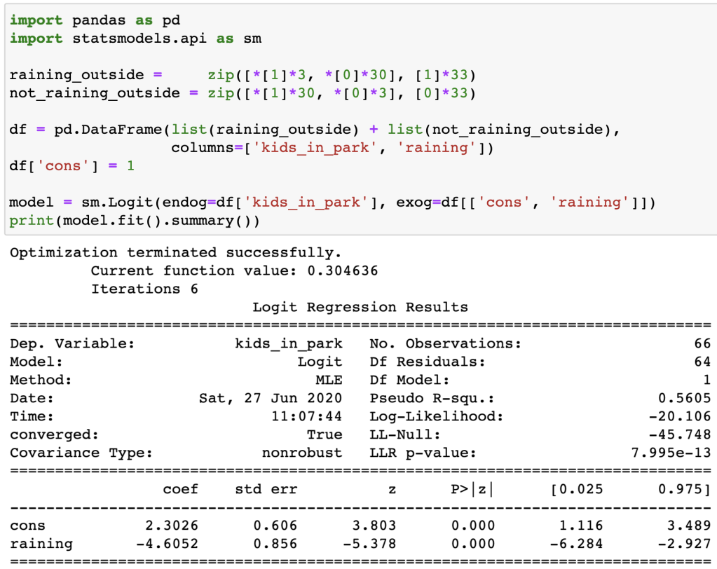
Most statistical software packages I’m aware of report the coefficients of a logistic regression in the logit form, i.e. as log odds ratios, as you can see above.

The coefficients are log odds ratios of the marginal effects of the variables in , and is the sum product of those marginal effects and their respective features, resulting in a log odds (not a ratio). And if you take , you return to a probability between 0 and 1.

(As a note: I’m not sure where to put this in the explanation, but while we’re on the topic: “logistic” is not synonymous with “sigmoidal;” logistic functions are a subset of all possible sigmoids. For example, normal CDFs, which are the inverse of probits, are also sigmoids.)

Logistic Regression is Not Fundamentally a Classification Algorithm

Classification is when you make a concrete determination of what category something is a part of. Binary classification involves two categories, and by the law of the excluded middle, that means binary classification is for determining whether something “is” or “is not” part of a single category. There either are children playing in the park today (1), or there are not (0).

Although the variable you are targeting in logistic regression is a classification, logistic regression does not actually individually classify things for you: it just gives you probabilities (or log odds ratios in the logit form). The only way logistic regression can actually classify stuff is if you apply a rule to the probability output. For example, you may round probabilities greater than or equal to 50% to 1, and probabilities less than 50% to 0, and that’s your classification.

That logistic regression is taught in machine learning courses as a classification algorithm leads to a lot of avoidable confusion because it is an extremely limited view of what logistic regression is.

Imagine you have a bucket of 100 apples. 80 of them are red, and 20 of them are green. Let’s say red corresponds to y=1 in your data, and green corresponds to y=0. If you have no way to identify apples other than the coefficient, i.e. , then your estimates for each row of data will be 0.8. Use the classification rule mentioned above– i.e. round to the nearest whole number– will make your fitted data be 1’s. Your model now says say all your apples are red.

Obviously this is silly because not all your apples are red. But does it matter? Well, it depends on the context. If you want to be simply maximize the probability you correctly identify an apple’s color when taking a guess on a single apple, then this is the best approach. If you want to know the total expected number of red apples within an out-of-sample population of apples, then this is a bad approach; you would rather sum the individual probabilities without rounding them to 0 or 1 first.

Let’s step away from apples for a moment and examine more concrete scenarios:

• Let’s say you have a bunch of bank transaction data and you’re trying to create a fraud detection system trained on perfectly accurate training data. In practice, fraud doesn’t happen much, so very few rows of data will ever achieve a ≥ 50% chance of fraud and round up to 1. But the cost of fraud is quite high. So if you see a 20% fraudulent transaction, it’s probably worth halting 4 non-fraudulent transactions if it means 1 fraudulent transaction on average gets stopped. So your actual classification cut-off will be 20%, not 100%. This is effectively an adjustment to the loss function, which should be made based on understanding the trade-offs associated with false positives and false negatives. Basically, you need to pick a point on your receiver operator curve (ROC) and apply that threshold, but you need external information outside of your model to decide which point makes the most sense (e.g. regulations, consumer satisfaction surveys).
• If you have a securitized portfolio of loans, you may want to know how certain attributes of the loan recipients affect the probability of default. You may then use a model fit on that old set of loan data on a new set of loan data to predict defaults. The way to do this is is to simply sum the probabilities of the new portfolio. One convenient property of binomials is that if you take the sum of the probability of a hit p and multiply by the sample size N, you get the average number of expected hits k. Some people accidentally confuse themselves into thinking, “no, you actually need to take one minus one minus the probability, to the power of…” what they are calculating is , not . If you flip a coin 50 times, on average it will be heads 25 times. It’s literally that simple, and you can even do this with logistic regression outputs. Don’t trick yourself into thinking it’s more complicated than it actually is.

Logistic regression as classification makes the most sense when you need to make discrete actionable decisions. In the case of fraud, you need to either accept the transaction, decline it, or accept the transaction but notify the bank customer that it looks suspicious. These are three possible decisions, each which can be classified. Similarly, email spam filters need to decide whether an email is spam (if yes, move to junk mail) or not (then keep in the inbox), which is also a discrete actionable decision that is fit for classification.

In the case of a portfolio of loans, what’s the classification problem, exactly? If these loans are securitized, you just want to know the total risk. Even on a loan-by-loan basis in the case of individual borrowers, you will probably still lend to someone– but when the credit risk is higher, you’ll just charge higher interest or require a higher down payment. This is not really a discrete decision, it is a continuous spectrum. It’s not a classification problem. Nevertheless, logistic regression was the correct model for the job. The fact that it’s often best to use logistic regression without rounding the outputs to 0 or 1 confounds many practicing data scientists.

Misguided Approaches To Ill-Defined Problems

I help teach a handful of people how to code as part of some projects I do on the side. I constantly emphasize making liberal use of Google to solve problems. One thing I always stress, though, is that Google can answer your questions in most circumstances, but it won’t tell you whether the question you’re asking is the right question.

One of the more dangerous Google searches you can do in the context of data science is to type “how to fix imbalanced data” into the search bar. Imbalanced data means that you have a lot of things in one bucket and very few things in other buckets.

The supposed problem of imbalanced data has been implicitly described three times in this blog post (apples, fraud, default risk), yet until this section I neither used the term “imbalanced data” nor have I used some of the proposed solutions you’ll see in these blog posts on Google, which often focus on “rebalancing” your dataset through resampling of the under-represented categories. I never proposed this solution because “imbalanced data” is not actually a major “problem” in the majority of circumstances in which people often think it’s a problem. Oftentimes, the problem is that people are butting heads with an extremely limited views of what they’re supposed to do in the context of supervised learning problems that contain a binary target variable. Just because your variable is binary, it doesn’t mean your needs to be.

I don’t mean to say that there aren’t contexts in which “rebalancing” your data is a fine way to optimize your model. There are contexts in which it is appropriate, but if your model is already FUBAR, then you probably aren’t encountering such a problem. Rebalancing solves problems when your sample data is a biased representation of the context in which the model will be practically used; or if a feature-rich model needs to pay extra-close attention to patterns that predict infrequent occurrences in a way that is not straightforwardly obviated by adjustments to the loss function. Otherwise, rebalancing represents marginal improvements at best. Yet Google is replete with blog posts suggesting this approach as if it’s a good solution to a common problem, and none of the writers of these posts warn the user that they probably need another approach. It is not a good solution and it is not a common “problem.” If data scientists had a better conceptual grasp of the difference between probability problems and classification problems, most of those blog posts might not exist.

---

June 28, 2020 revisions: Thank you for the feedback to all that have provided it. I’ve made a couple small changes.

First, two conceptual errors in my description of logit. I mistakenly included error terms in my logistic regression LaTeX. Logistic regressions don’t have error terms because probabilities themselves are, in a sense, errors. Thank you to Cameron Patrick (@camjpatrick) for pointing this error out (pun intended). Also, Darren Dahly (@statsepi) pointed out that it’s a mistake to refer to Logit(y) as a log odds ratio, just log odds. I have a sense of humor and can appreciate the irony in making some conceptual mistakes in a blog post with an inflammatory title such as this.

Second, my section on rebalancing data deserved more nuance and a fairer treatment of the subject; I’ve tinkered with some of the verbiage to reflect that, although it mostly preserves the same tone. My original discussion seemed to suggest that rebalancing simply isn’t a tool you should employ except in “weird situations.” What it should have said is: rebalancing data is not a substitute for making sound judgment calls about your loss function. Rebalancing as classification panacea is a genuine mistake and a lot of data scientists make it. My first exposure to the idea of “rebalancing” data in the ML sense was nearly a year ago in the context of some analysts I was helping, who mistakenly conceptualized a risk-measurement problem as a classification problem. They thought the solution to their model classifying 100% of observations as a 0 was to rebalance the data, when the more obvious solution was to use a lower threshold or avoid binary classification entirely.

There are, however, a fair number of generalized cases where rebalancing can increase your AUC slightly but assuredly in classification problems, and not just as a substitute for bad loss functions. Specifically, rebalancing can make minor improvements to the AUC when your features are normally distributed but the covariance matrix of those features conditional on y=0 differs from the covariance matrix conditional on y=1. Which is actually a pretty common occurrence in real data. Thank you to Jake Westfall (@CookieSci) who pointed me to this paper that explains the math behind it.

This doesn’t negate the main point of this section, though: most people who do venerable work on risk-based problems for a living don’t typically encounter situations in which imbalance is a fundamental problem in their modeling because they’re not using raw classification accuracy as their metric of choice.