The Size of Tracing Data

Sep 6, 2020 | tracing

Tracing is an invaluable technique for capturing data about rare events. Based on a heuristic that you as the application developer likely know best, you wrap interesting sections of code with the following:

long start = System.nanoTime();
doStuff();
long duration = System.nanoTime() - start;
report(TIMER_NAME, duration);

Wrapping a contended lock in this fashion can be especially revealing. The majority of the data captured will be garbage, but this will capture outliers in a way a profiler won’t. Imagine capturing it all, naïvely, as a stream of named durations. Assuming a zero overhead storage format, this will cost 8 + TIMER_NAME.length() bytes per row. The timer name is almost certainly representable in ASCII, so requires one byte per character, but will probably be “fully qualified” and quite long, say 50 characters. If you record 20,000 of these per second, you will generate roughly 1.1MB/s. You can be smarter and dictionary encode the metric names (replace them with an integer encoding) and even using a naïve 4 bytes per name gets you down to 235KB/s, but 156KB/s is the floor. This is quite a lot of data, and it’s just for one traced function.

An obvious solution is to use a histogram, which requires quantisation into time buckets, for instance HdrHistogram. In practice, the majority of measurements will fall into relatively few time buckets, and at some point there will be no more allocation at all, except for the occasional snapshot of the histogram. It’s possible to use fewer bits for the boring measurements than for the outliers. In the usual case, the buckets covering commonly observed values share integer prefixes, with very low counts in buckets containing extreme values. This allows for prefix compression - for instance see the packed variant of HdrHistogram. DDSketches collapses common buckets and uses an interpolation function to produce approximate quantiles with low error.

To demonstrate the benefits to be reaped by exploiting properties of the data ensemble, I simulated accesses to a lock from 20000 competing requests.

  private static double generatePoisson(double rate) {
    return (-1.0 / rate) * Math.log(ThreadLocalRandom.current().nextDouble());
  }

  private static double generateLogNormal(double mean, double stdDev) {
    return Math.exp(ThreadLocalRandom.current().nextGaussian() * stdDev + mean);
  }

  private static long toDuration(double rv) {
    return Math.max(0, (long) rv);
  }

  private static long[] generateDurations(int count,
                                          double frequentRate,
                                          double frequentMean,
                                          double frequentStdDev,
                                          double infrequentRate,
                                          double infrequentMean,
                                          double infrequentStdDev) {
    long[] durations = new long[count];
    double nextFrequent = generatePoisson(frequentRate);
    double nextInfrequent = generatePoisson(infrequentRate);
    int counter = 0;
    while (counter < durations.length) {
      double rv;
      if (nextFrequent < nextInfrequent) {
        rv = generateLogNormal(frequentMean, frequentStdDev);
        nextFrequent += generatePoisson(frequentRate);
      } else {
        rv = generateLogNormal(infrequentMean, infrequentStdDev);
        nextInfrequent += generatePoisson(infrequentRate);
      }
      durations[counter++] = toDuration(rv);
    }
    return durations;
  }

The lock is frequently uncontended. Uncontended accesses, which themselves have lognormally distributed durations, arrive as a poisson process with high intensity. Contended accesses arrive less frequently as a poisson process with lower intensity, and the durations (i.e. including time waiting for the lock) have lognormal distribution with higher mean and variance.

    long[] durations = generateDurations(20000, 0.9, 1.0, 0.01, 0.01, 10.0, 0.5);

    DDSketch denseDDSketch = DDSketch.fast(0.001);
    DDSketch sparseDDSketch = DDSketch.memoryOptimal(0.001);
    PackedHistogram packedHistogram = new PackedHistogram(30 * 1000_000_000L, 3);
    Histogram histogram = new Histogram(30 * 1000_000_000L, 3);

    for (long duration : durations) {
      denseDDSketch.accept(duration);
      sparseDDSketch.accept(duration);
      packedHistogram.recordValue(duration);
      histogram.recordValue(duration);
    }

Here is a visualisation of the distribution

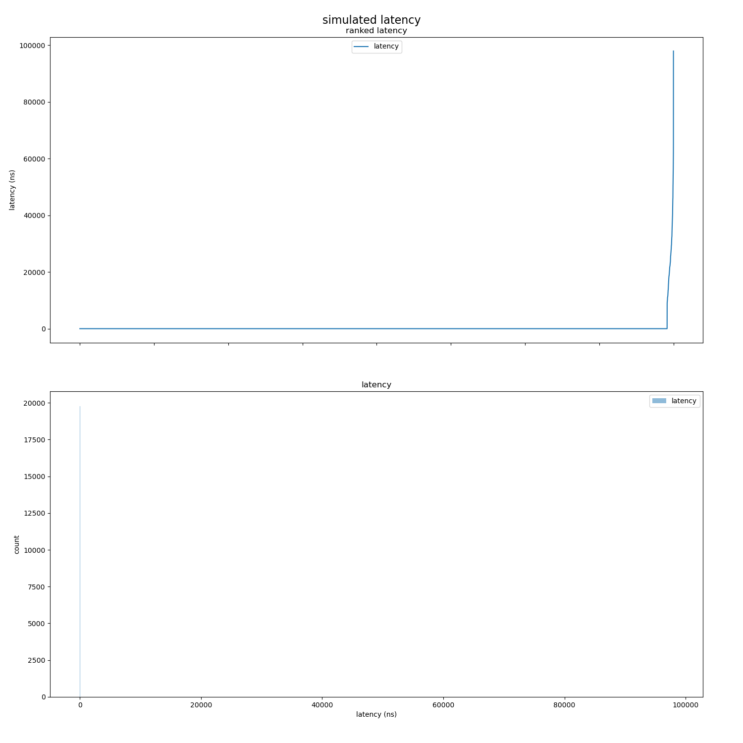
To evaluate the true cost of shipping this data at 20000 requests per second, you really need to serialize it, and whilst HdrHistogram supports this, DDSketch doesn’t (yet?), so I compared the in memory footprints using JOL as a comparable proxy. The problem with comparing the in-memory representation is that things like padding for false sharing evasion contributes to the cost, and conversely, there may be structural sharing not possible on disk. DDSketch’s Java implementation is still in its early days and isn’t optimal (the sparse implementation is backed by a NavigableMap<Integer, Long>…), but it still does a lot better than the naïve array of durations. The sizes below ignore any labeling/names.

Storage Total Size (KB) HdrHistogram (dense) 209 Array 156 DDSketch (dense) 61 DDSketch (sparse) 41 HdrHistogram (sparse) 3

There is no such thing as a free lunch: histograms lose information about when the events occurred. If you want to change the tracing function to record the start time as follows

long epochStart = MILLISECONDS.toNanos(System.currentTimeMillis());
long epochStartNanoTime = System.nanoTime();
...
long start = System.nanoTime();
doStuff();
long duration = System.nanoTime() - start;
report(TIMER_NAME,  start + epochStart - epochStartNanoTime, duration);

Then histograms are no longer an option, but it doesn’t need to take hundreds of kilobytes per second, and ensemble properties can be exploited to reduce the size. First of all, the timestamps are monotonic, and can be represented by offsets relative to the start of an epoch. Then, these offsets are themselves monotonic. Further, if we can guarantee the epochs are shorter than a few seconds, the offsets need at most 32 bits, and can be safely cast to int. Over 99% of the durations were uncontended accesses, and are virtually the same value, then there are very few long durations. This is an artifact of the process which generates the data, and can be exploited using integer compression. Even the long durations don’t need 64 bits each, and can be safely cast to int.

JavaFastPFOR is capable of exploiting these patterns so you can capture all the data without it getting too big. It’s also extremely fast, both to encode and decode; much faster than general purpose compression.

    int[][] durationsWithStartTimes = generateDurationsWithStartTimes(20000, 0.9, 1.0, 0.01, 0.01, 10.0, 0.5);
    IntegratedIntCompressor compressor = new IntegratedIntCompressor();
    int[] compressedDurations = compressor.compress(durationsWithStartTimes[0]);
    int[] compressedStartTimes = compressor.compress(durationsWithStartTimes[1]);

This is cheating in the kind of way you can cheat when you’re close to the problem. If you’re tracing lock accesses, it’s perfectly reasonable to assume everything takes less than 4 billion nanoseconds. For the naïve baseline, we can employ the same trick for the durations, but without a frame of reference, 64 bits are required for each of the timestamps. To record a second’s worth of data at 20K requests per second, the space required is

Storage Total Size (KB) long durations, long timestamps 312 int durations, long timestamps 274 FastPFOR 56

Having a frame of reference just makes such a difference to this kind of data.

Next time, we’ll take a look at the spatial overhead imposed by the open tracing standard opentelemetry!