Combining knowledge graphs, quickly and accurately

Knowledge graphs are a way of representing information that can capture complex relationships more easily than conventional databases. At Amazon, we use knowledge graphs to represent the hierarchical relationships between product types on amazon.com; the relationships between creators and content on Amazon Music and Prime Video; and general information for Alexa’s question-answering service — among other things.

Expanding a knowledge graph often involves integrating it with another knowledge graph. But different graphs may use different terms for the same entities, which can lead to errors and inconsistencies during integration. Hence the need for automated techniques of entity alignment , or determining which elements of different graphs refer to the same entities.

In apaper accepted to the Web Conference, my colleagues and I describe a new entity alignment technique that factors in information about the graph in the vicinity of the entity name. In tests involving the integration of two movie databases, our system improved upon the best-performing of ten baseline systems by 10% on a metric called area under the precision-recall curve (PRAUC), which evaluates the trade-off between true-positive and true-negative rates.

Despite our system’s improved performance, it remains highly computationally efficient. One of the baseline systems we used for comparison is a neural-network-based system called DeepMatcher, which was specifically designed with scalability in mind. On two tasks, involving movie databases and music databases, our system reduced training time by 95% compared to DeepMatcher, while offering enormous improvements in PRAUC.

A graph is a mathematical object that consists of nodes, usually depicted as circles, and edges, usually depicted as line segments connecting the circles. Network diagrams, organizational charts, and flow charts are familiar examples of graphs.

Our work specifically addresses the problem of merging multi-type knowledge graphs, or knowledge graphs whose nodes represent more than one type of entity. For instance, in the movie data sets we worked with, a node might represent an actor, a director, a film, a film genre, and so on. Edges represented the relationships between entities — acted in, directed, wrote, and so on.

This example illustrates the challenge of entity alignment. IMDB lists the writer of the movie Don’t Stop Dreaming as Aditya Raj, but the (now defunct) Freebase database lists him as Aditya Raj Kapoor. Are they the same person?

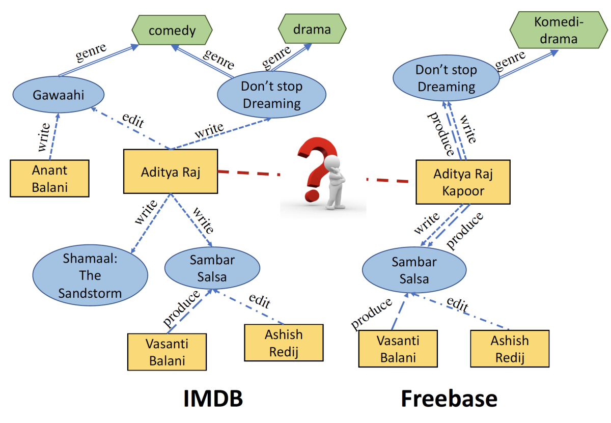
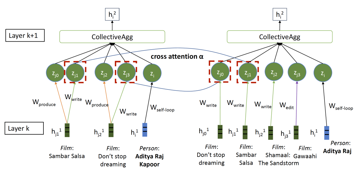
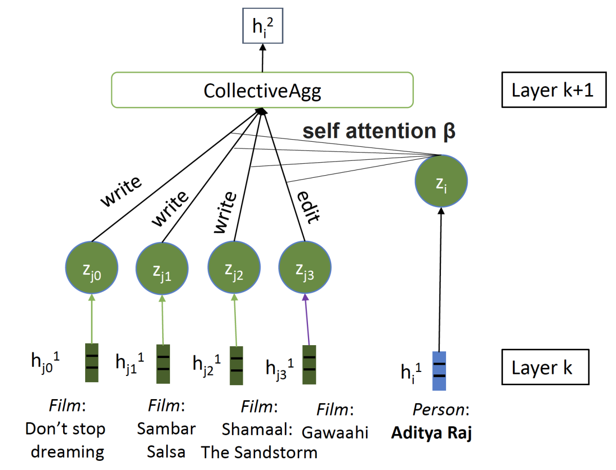
Our system is an example of a graph neural network, a type of neural network that has recently become popular for graph-related tasks. To get a sense for how it works, consider the Freebase example above, which includes what we call the “neighborhood” of the node representing Aditya Raj Kapoor. This is a two-hop local graph, meaning that it conrtains the nodes connected to Kapoor (one hop) and the nodes connected to them (two hops), but it doesn’t fan out any farther through the knowledge graph. The neighborhood thus consists of six nodes.

With a standard graph neural network (GNN), the first step — known as the level-0 step — is to embed each of the nodes, or convert it to a fixed-length vector representation. That representation is intended to capture information about node attributes useful for the network’s task — in this case, entity alignment — and it’s learned during the network’s training.

Next, in the level-1 step, the network considers the central node (here, Aditya Raj Kapoor) and the nodes one hop away from it ( Don’t Stop Dreaming and Sambar Salsa ). For each of these nodes, it produces a new embedding, which consists of the node's level-0 embedding concatenated with the sum of its immediate neighbors' level-0 embeddings.

At the level-2 step — the final step in a two-hop network — the network produces a new embedding for the central node, which consists of that node’s level-1 embedding concatenated with the summation of the level-1 embeddings of its immediate neighbors.

In our example, this process compresses the entire six-node neighborhood graph from the Freebase database into a single vector. It would do the same with the ten-node neighborhood graph from IMDB, and comparing the vectors is the basis for the network’s decision about whether or not the entities at the centers of the graphs — Aditya Raj and Aditya Raj Kapoor — are the same.

This is the standard implementation of the GNN for the entity alignment problem. Unfortunately, in our experiments, it performed terribly. So we made two significant modifications.

The first was a cross-graph attention mechanism. During the level-1 and level-2 aggregation stages, when the network sums the embeddings of each node’s neighbors, it weights those sums based on a comparison with the other graph.

In our example, that means that during the level-1 and level-2 aggregations, the nodes Don’t Stop Dreaming and Sambar Salsa , which show up in both the IMDB and Freebase graphs, will get greater weight than Gawaahi and Shamaal , which show up only in IMDB.

In this example, our cross-graph attention mechanism (blue lines) gives added weight (dotted red lines) to the embeddings of entities shared between neighborhood graphs.

The cross-graph attention mechanism thus emphasizes correspondences between the graphs and de-emphasizes differences. After all, the differences between the graphs is why it’s useful to combine their information in the first place.

The original version of “Radioactive” and the remix are distinct tracks, but they share so many attributes that a naïve entity alignment system might misclassify them as identical.

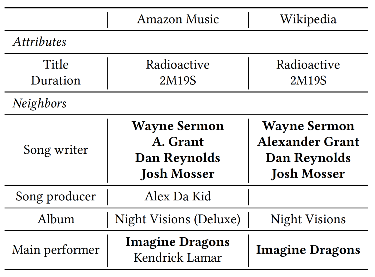
This approach has one major problem, however: sometimes the differences between graphs matter more than their correspondences. Consider the example at left, which compares two different versions of Imagine Dragons’ hit “Radioactive”, the original album cut and the remix featuring Kendrick Lamar.

Here, the cross-graph attention mechanism might overweight the many similarities between the two tracks and underweight the key difference: the main performer. So our network also includes a self-attention mechanism .

The application of our self-attention mechanism in our running example involving Aditya Raj.

During training, the self-attention mechanism learns which attributes of an entity are most important for distinguishing it from entities that look similar. In this case, it would learn that many distinct recordings may share the same songwriter or songwriters; what distinguishes them is the performer.

These two modifications are chiefly responsible for the improved performance of our model versus the ten baselines we compared it with.

Finally, a quick remark about one of the several techniques we used to increase our model’s computational efficiency. Although, for purposes of entity alignment, we compare two-hop neighborhoods, we don’t necessarily include a given entity’s entire two-hop neighborhood. We impose a cap on the number of nodes included in the neighborhood, and to select nodes for inclusion, we use weighted sampling.

The sample weights have an inverse relationship to the number of neighbor nodes that share the same relationship to the node of interest. So, for instance, a movie might have dozens of actors but only one director. In that case, our method would have a much higher chance of including the director node in our sampled neighborhood than it would of including any given actor node. Restricting the neighborhood size in this way prevents our method’s computational complexity from getting out of hand.